
CMPS 251 Homework Assignment 3 Solution, Fall 2015
American University of Beirut · Numerical Computing · 7 pages · with solution

More CMPS 251 files
- Homework Assignment 4 · Fall 2015HomeworkView
- Homework Assignment 4 Solution · Fall 2015Homework · with solutionView
- Homework Assignment 3 · Fall 2015HomeworkView
- Homework Assignment 5 · Fall 2015HomeworkView
- Homework Assignment 2 Solution · Fall 2015Homework · with solutionView
- Homework Assignment 1 · Fall 2015HomeworkView
- Homework Assignment 1 Solution · Fall 2015Homework · with solutionView
- Homework Assignment 2 · Fall 2015HomeworkView
Show the text of this homework
CMPS 251
Assignment 3‐ Solution
Problem 1
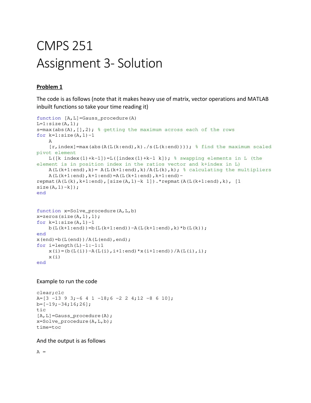
The code is as follows (note that it makes heavy use of matrix, vector operations and MATLAB
inbuilt functions so take your time reading it)
function [A,L]=Gauss_procedure(A)
L=1:size(A,1);
s=max(abs(A),[],2); % getting the maximum across each of the rows
for k=1:size(A,1)-1
A
[r,index]=max(abs(A(L(k:end),k)./s(L(k:end)))); % find the maximum scaled
pivot element
L([k index(1)+k-1])=L([index(1)+k-1 k]); % swapping elements in L (the
element is in position index in the ratios vector and k+index in L)
A(L(k+1:end),k)= A(L(k+1:end),k)/A(L(k),k); % calculating the multipliers
A(L(k+1:end),k+1:end)=A(L(k+1:end),k+1:end)-
repmat(A(L(k),k+1:end),[size(A,1)-k 1]).*repmat(A(L(k+1:end),k), [1
size(A,1)-k]);
end
function x=Solve_procedure(A,L,b)
x=zeros(size(A,1),1);
for k=1:size(A,1)-1
b(L(k+1:end))=b(L(k+1:end))-A(L(k+1:end),k)*b(L(k));
end
x(end)=b(L(end))/A(L(end),end);
for i=length(L)-1:-1:1
x(i)=(b(L(i))-A(L(i),i+1:end)*x(i+1:end))/A(L(i),i);
x(i)
end
Example to run the code
clear;clc
A=[3 -13 9 3;-6 4 1 -18;6 -2 2 4;12 -8 6 10];
b=[-19;-34;16;26];
tic
[A,L]=Gauss_procedure(A);
x=Solve_procedure(A,L,b);
time=toc
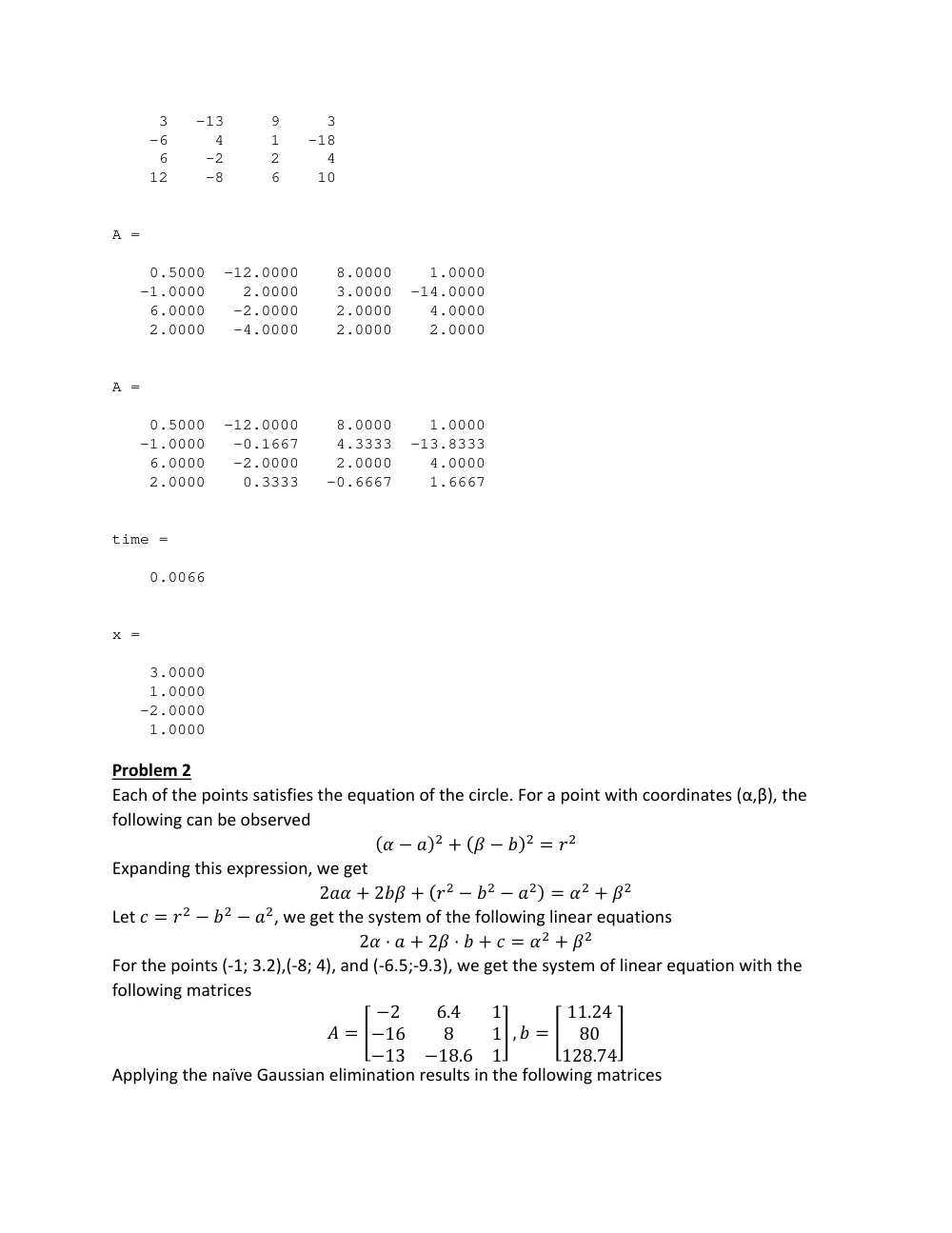
And the output is as follows
A =
3 -13 9 3
-6 4 1 -18
6 -2 2 4
12 -8 6 10
A =
0.5000 -12.0000 8.0000 1.0000
-1.0000 2.0000 3.0000 -14.0000
6.0000 -2.0000 2.0000 4.0000
2.0000 -4.0000 2.0000 2.0000
A =
0.5000 -12.0000 8.0000 1.0000
-1.0000 -0.1667 4.3333 -13.8333
6.0000 -2.0000 2.0000 4.0000
2.0000 0.3333 -0.6667 1.6667
time =
0.0066
x =
3.0000
1.0000
-2.0000
1.0000
Problem 2
Each of the points satisfies the equation of the circle. For a point with coordinates (α,β), the
following can be observed
�� � ��� � �� � ��� � ��
Expanding this expression, we get
2�� � 2�� � ��� � �� � ��� � �� � ��
Let � � �� � �� � ��, we get the system of the following linear equations
2� ⋅ � � 2� ⋅ � � � � �� � ��
For the points (‐1; 3.2),(‐8; 4), and (‐6.5;‐9.3), we get the system of linear equation with the
following matrices
� � �
�2
6.4
1
�16
8
1
�13
�18.6
1
� , � � �
11.24
80
128.74
�
Applying the naïve Gaussian elimination results in the following matrices
� � �
�2
6.4
1
0
�43.2
�7
0
0
4.2546
� , � � �
11.24
�9.92
69.4637
�
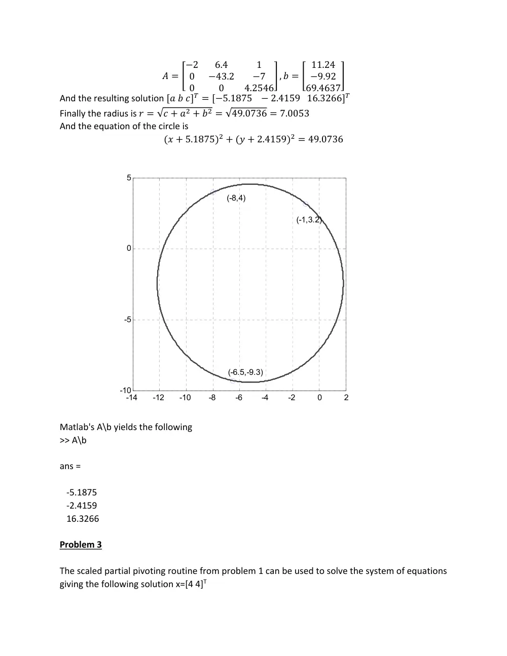
And the resulting solution �� � ��� � ��5.1875 � 2.4159 16.3266��
Finally the radius is � � √� � �� � �� � √49.0736 � 7.0053
And the equation of the circle is
�� � 5.1875�� � �� � 2.4159�� � 49.0736
Matlab's A\b yields the following
>> A\b
ans =
‐5.1875
‐2.4159
16.3266
Problem 3
The scaled partial pivoting routine from problem 1 can be used to solve the system of equations
giving the following solution x=[4 4]T
-14
-12
-10
-8
-6
-4
-2
0
2
-10
-5
0
5
(-6.5,-9.3)
(-8,4)
(-1,3.2)
Now, by perturbating the matrix A and the vector b as required in the assignment, the new
solution becomes [3.98 4.04]T. By trying for instance to perturbate A without perturbating b,
the solution becomes [2.02 6.91]T
We can see that the system of equations is sensitive to the slightest changes in the coefficients.
We suspect that the matrix is ill‐conditioned.
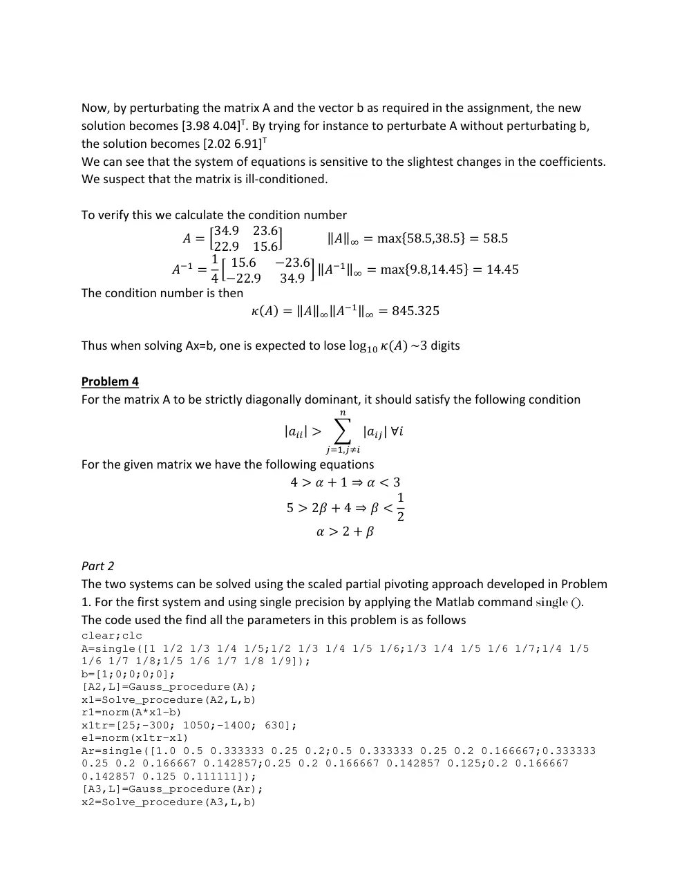
To verify this we calculate the condition number
� � �34.9
23.6
22.9
15.6� ‖�‖� � max�58.5,38.5� � 58.5
��� � 1
4 � 15.6
�23.6
�22.9
34.9 � ‖���‖� � max�9.8,14.45� � 14.45
The condition number is then
���� � ‖�‖�‖���‖� � 845.325
Thus when solving Ax=b, one is expected to lose log�� ���� ~3 digits
Problem 4
For the matrix A to be strictly diagonally dominant, it should satisfy the following condition
|���| �
� |���| ∀�
�
���,���
For the given matrix we have the following equations
4 � � � 1 ⇒ � � 3
5 � 2� � 4 ⇒ � � 1
2
� � 2 � �
Part 2
The two systems can be solved using the scaled partial pivoting approach developed in Problem
1. For the first system and using single precision by applying the Matlab command single ().
The code used the find all the parameters in this problem is as follows
clear;clc
A=single([1 1/2 1/3 1/4 1/5;1/2 1/3 1/4 1/5 1/6;1/3 1/4 1/5 1/6 1/7;1/4 1/5
1/6 1/7 1/8;1/5 1/6 1/7 1/8 1/9]);
b=[1;0;0;0;0];
[A2,L]=Gauss_procedure(A);
x1=Solve_procedure(A2,L,b)
r1=norm(A*x1-b)
x1tr=[25;-300; 1050;-1400; 630];
e1=norm(x1tr-x1)
Ar=single([1.0 0.5 0.333333 0.25 0.2;0.5 0.333333 0.25 0.2 0.166667;0.333333
0.25 0.2 0.166667 0.142857;0.25 0.2 0.166667 0.142857 0.125;0.2 0.166667
0.142857 0.125 0.111111]);
[A3,L]=Gauss_procedure(Ar);
x2=Solve_procedure(A3,L,b)
r2=norm(Ar*x2-b)
x2tr=[26.9314;-336.018; 1205.11;-1634.03;744.411];
e2=norm(x2tr-x2)
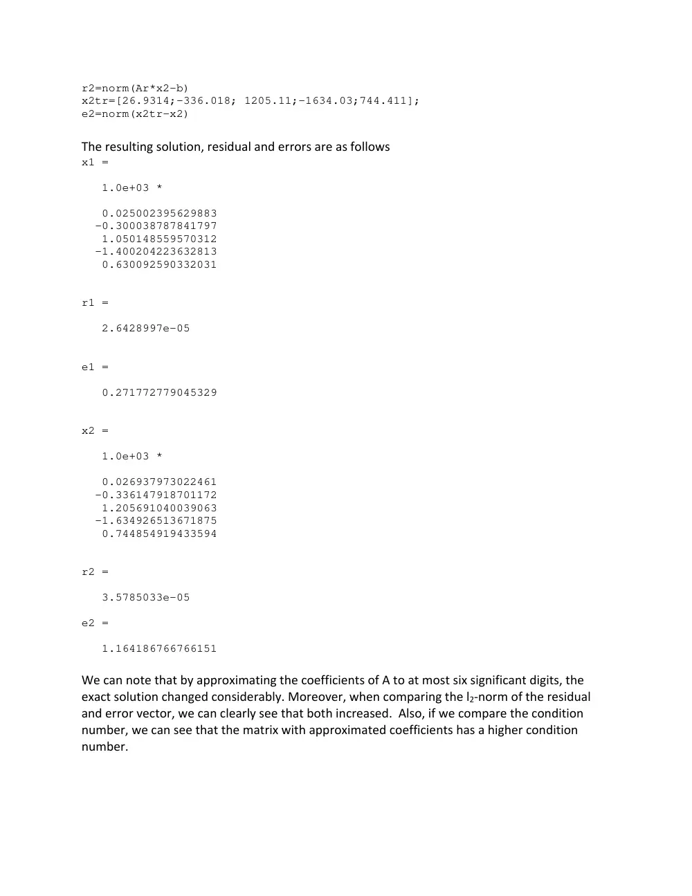
The resulting solution, residual and errors are as follows
x1 =
1.0e+03 *
0.025002395629883
-0.300038787841797
1.050148559570312
-1.400204223632813
0.630092590332031
r1 =
2.6428997e-05
e1 =
0.271772779045329
x2 =
1.0e+03 *
0.026937973022461
-0.336147918701172
1.205691040039063
-1.634926513671875
0.744854919433594
r2 =
3.5785033e-05
e2 =
1.164186766766151
We can note that by approximating the coefficients of A to at most six significant digits, the
exact solution changed considerably. Moreover, when comparing the l2‐norm of the residual
and error vector, we can clearly see that both increased. Also, if we compare the condition
number, we can see that the matrix with approximated coefficients has a higher condition
number.
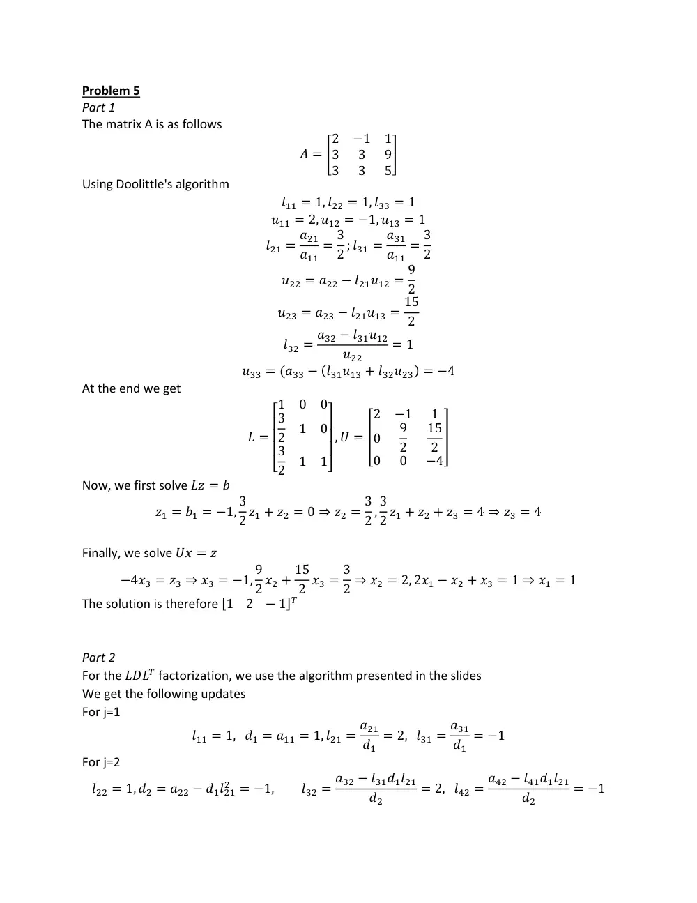
Problem 5
Part 1
The matrix A is as follows
� � �
2
�1
1
3
3
9
3
3
5
�
Using Doolittle's algorithm
��� � 1, ��� � 1, ��� � 1
��� � 2, ��� � �1, ��� � 1
��� � ���
���
� 3
2 ; ��� � ���
���
� 3
2
��� � ��� � ������ � 9
2
��� � ��� � ������ � 15
2
��� � ��� � ������
���
� 1
��� � ���� � ������� � ������� � �4
At the end we get
� �
�
�
�
�
�1
0
0
3
2
1
0
3
2
1
1�
�
�
�
�
, � � �
2
�1
1
0
9
2
15
2
0
0
�4
�
Now, we first solve �� � �
�� � �� � �1, 3
2 �� � �� � 0 ⇒ �� � 3
2 , 3
2 �� � �� � �� � 4 ⇒ �� � 4
Finally, we solve �� � �
�4�� � �� ⇒ �� � �1, 9
2 �� � 15
2 �� � 3
2 ⇒ �� � 2, 2�� � �� � �� � 1 ⇒ �� � 1
The solution is therefore �1 2 � 1��
Part 2
For the ���� factorization, we use the algorithm presented in the slides
We get the following updates
For j=1
��� � 1, �� � ��� � 1, ��� � ���
��
� 2, ��� � ���
��
� �1
For j=2
��� � 1, �� � ��� � �����
� � �1,
��� � ��� � ��������
��
� 2, ��� � ��� � ��������
��
� �1
For j=3
��� � 1, �� � ��� � ������
� � �����
� � � 2, ��� � ��� � ��������� � ���������
��
� 1
for j=4
��� � 1, �� � ��� � ������
� � �����
� � �����
� � � �2
Finally the L and D matrices are as follows
� � �
1
0
2
1
�1
2
0
0
0
0
1
0
1
�1 1
1
� , � � �
1
0
0
�1
0
0
0
0
0
0
2
0
0
0 0
�2
�
For the Cholesky factorization, again we use the algorithm in the slides
For k=1
��� � ���� � √6,
��� � ���
���
� 15
√6
, ��� � ���
���
� 55
√6
For k=2
��� � ���� � ���
� � �105
6 , ��� � ��� � ������
���
� 525√630
630
For k=3
��� � ���� � ���
� � ���
� � �34860
630
Taking approximations, the resulting matrix L is as follows
� � �
2.4495
0
0
6.1237
4.1833
0
22.4537
20.9165
7.4386
�
Part 3
For this matrix, we need to permute rows 1 and 2 to be able to do Gaussian elimination. The
permutation matrix is therefore as follows
� � �
0
1
0
1
0
0
0
0
1
�