EECE 340 Homework 1 Solution, Spring 2015

EECE 340 Signals and Systems Jun . 10, 2015 American University of Beirut, Summer 2014–2015 Handout #3 Problem Set 1 – Solutions Problem 1.1 1) Our system here may be described as follows: Denoting by y[n] the amount of money our neighbor has at ABB at the end of year n, and by x[n] the amount she deposits/withdraws during year n, y[n] = (1 + r)y[n − 1] + x[n], where the interest rate is r = 0.04. We naturally assume that the system is initially at rest, and at time “0”, x[0] = 1000000 − 54000 and subsequently every year after that x[n] = −54000. Right away, we note that the modeling could have been done differently with an equally valid –maybe even more sensible– logic. The money the neighbor needs to live during a particular year is “charged” on accounts and the accounts are settled at the end of the year after she has incurred interest at ABB. Equivalently, x[0] = 1000000. Both models and other sensible ones are equally valid, and in this solution we adopt the first. 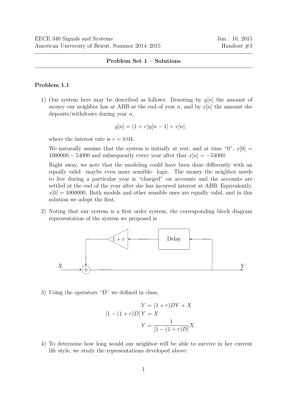2) Noting that our system is a first order system, the corresponding block diagram representation of the system we proposed is ✲ X + ❄ ✲Y ✛ Delay ✛ 1 + r 3) Using the operators “D” we defined in class, Y = (1 + r)DY + X [1 − (1 + r)D] Y = X Y = 1 [1 − (1 + r)D]X. 4) To determine how long would our neighbor will be able to survive in her current life style, we study the representations developed above: 1 – The block diagram is useful when we study the system along with other – possibly interacting– systems, and will not be probably useful to answer the question. – The representation with system functions using the “D” operator was very handy when it comes to determine the impulse response of the system. How- ever, in our model the input is not an impulse and this representations is not YET useful. – The only method we have seen to be appropriate to answer the question is through the difference equations, which we decide to use for the remainder of this question. 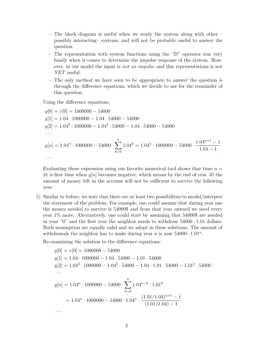Using the difference equations, y[0] = x[0] = 1000000 − 54000 y[1] = 1.04 · 1000000 − 1.04 · 54000 − 54000 y[2] = 1.042 · 1000000 − 1.042 · 54000 − 1.04 · 54000 − 54000 · · · y[n] = 1.04n · 1000000 − 54000 · n � k=0 1.04k = 1.04n · 1000000 − 54000 · 1.04n+1 − 1 1.04 − 1 · · · Evaluating these expression using our favorite numerical tool shows that time n = 31 is first time when y[n] becomes negative, which means by the end of year 30 the amount of money left in the account will not be sufficient to survive the following year. 5) Similar to before, we note that there are at least two possibilities to model/interpret the statement of the problem: For example, one could assume that during year one the money needed to survive is 54000$ and from that year onward we need every year 1% more. Alternatively, one could start by assuming that 54000$ are needed in year “0” and the first year the neighbor needs to withdraw 54000 · 1.01 dollars. Both assumption are equally valid and we adopt in these solutions: The amount of withdrawals the neighbor has to make during year n is now 54000 · 1.01n. Re-examining the solution to the difference equations: y[0] = x[0] = 1000000 − 54000 y[1] = 1.04 · 1000000 − 1.04 · 54000 − 1.01 · 54000 y[2] = 1.042 · 1000000 − 1.042 · 54000 − 1.04 · 1.01 · 54000 − 1.012 · 54000 · · · y[n] = 1.04n · 1000000 − 54000 · n � k=0 1.04n−k · 1.01k = 1.04n · 1000000 − 54000 · 1.04n · (1.01/1.04)n+1 − 1 (1.01/1.04) − 1 · · · 2 Evaluating these shows that time n = 26 is first time when y[n] becomes negative, which means by the end of year 25 the amount of money left in the account will not be sufficient to survive the following year. Problem 1.2 1) The unit-sample or impulse defined in class is an even signal, indeed, x[−n] = x[n] for all integers. 2) Let x[n] be a signal that is both even and odd. Examining the value at zero, x[0] = −x[0] because it is odd and hence x[0] = 0. Actually, any odd signal has to be equal to zero at time 0. Additionally, because it is even x[−n] = x[n] for any n ̸= 0. Being also odd means that x[−n] = −x[n] for any such n. Therefore, x[n] = −x[n] = 0. In conclusion, the only signal that is both even and odd is the all zero signal. 3) It is possible to have a signal that is neither such as x[0] = 1, x[1] = 1, x[n] = 0 for all other values of n. This signal is clearly not odd because it is not zero at time n = 0 and it is not even because x[−1] = 0 ̸= x[1] = 1. 4) If we define xe[n] = 1 2 [x[n] + x[−n]] , then xe[n] is even: xe[−n] = 1 2 [x[−n] + x[n]] = xe[n], since addition is commutative. 6) If we were to decompose every signal into an even and an odd part, x[n] = xe[n] + xo[n], by computing the difference xo[n] = 1 2 [x[−n] − x[n]], which indeed an odd signal as xo[−n] = −xo[n]. 5) This decomposition into a sum of even and odd signals is unique. Indeed, one can make the following observations: (a) Let us decompose the “all-zero” signal 0[n] as 0[n] = e[n] + o[n]. The odd signal o[n] is zero at n = 0 by what was derived above. Assume that this odd signal is not the all zero signal, i.e., o[l] = c ̸= 0 for some l ̸= 0. 3 Since the sum is zero, e[l] = −c. Now observe the value of these signals at n = −l, 0 = 0[−l] = e[−l] + o[−l] = e[l] − o[−l] = −c − c = −2c, which implies that c = 0 which is a contradiction. In conclusion, 0[n] can be decomposed uniquely into 0[n] = 0[n] + 0[n]. (b) Now let x[n] be any signal and assume that it can be decomposed into an even and odd function in two different ways x[n] = e1[n] + o1[n]; x[n] = e2[n] + o2[n]. Taking the difference, 0[n] = (e1 − e2)[n] + (o1 − o2)[n]. Now since the linear combination of two even/odd signals is even/odd respec- tively, and since the decomposition of 0[n] is unique, then necessarily e1 = e2 & o1 = o2. 7) The even part of x[n] is e[n] = 1 2(x[n] + x[−n]) = 1 2 ��1 3 �n + �1 3 �−n� = cosh � n ln 1 3 � . Its odd part is o[n] = 1 2(x[n] − x[−n]) = 1 2 ��1 3 �n − �1 3 �−n� = sinh � n ln 1 3 � . 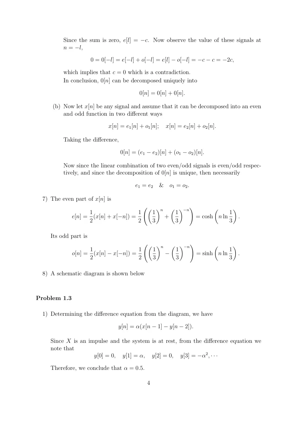8) A schematic diagram is shown below Problem 1.3 1) Determining the difference equation from the diagram, we have y[n] = α(x[n − 1] − y[n − 2]). Since X is an impulse and the system is at rest, from the difference equation we note that y[0] = 0, y[1] = α, y[2] = 0, y[3] = −α2, · · · Therefore, we conclude that α = 0.5. 4 −6 −4 −2 0 2 4 6 −400 −300 −200 −100 0 100 200 300 400 2) The system does not have a finite impulse response based on what we identified earlier. Indeed, we claim that y[n] = � (−1)(n−1)/2α(n+1)/2 n is positive and odd 0 o.w. We prove the claim by induction: (a) It is true for n = 0, 1. (b) Assume it is true up to n−1 ≥ 1 and we prove that this implies that it is true for n. If n is even then both x[n − 1] and y[n − 2] are zero. If n is odd, then x[n − 1] = 0 and y[n] = −αy[n − 2] = −(−1)(n−3)/2αα(n−1)/2 = (−1)(n−1)/2α(n+1)/2. Finally, since α is positive, then y[n] is non-zero for arbitrarily large indices n and y[n] is not finite length. Problem 1.4 5 Since, 1 (1 − α)2 = (1 − α)−2, 1 (1 − α)2 = (1 − α)−2 = 1 + 2α + (−2)(−3) 2! α2 + (−2)(−3)(−4) 3! α3 + · · · = 1 + 2α + 3α2 + 4α3 + · · · + (n + 1)αn + · · · = ∞ � n=0 (n + 1)αn, which converges whenever |α| < 1. 6