EECE 340 Homework 3 Solution, Spring 2016

AMERICAN UNIVERSITY OF BEIRUT ELECTRICAL AND COMPUTER ENGINEERING DEPARTMENT EECE 340 Homework III – Laplace Solution Problem 1 The signal x1(t), shown below, is the input of an LTI system whose impulse response y1(t) is also shown below. Determine the output signal. 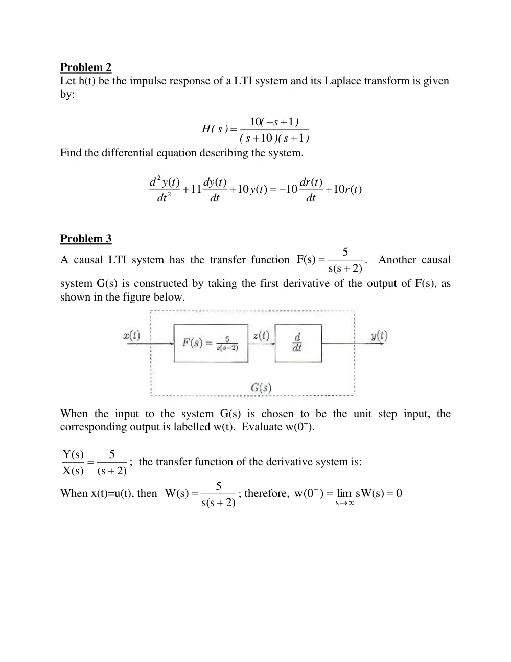 s  s e e s s X      2 3 1 1( )  s  s s e e e s s Y 3 2 2 1 3 3 1 1 ( )          s  s s s s e e e e s e X s Y s s Y 4 3 2 3 1 1 2 9 16 6 14 1 ( ) ( ) ( )                                  4) ( 4) 2( 3) ( 3) ( 9 2) ( 2) 16( )1 ( )1 14( ( ) 6 )1 ( )1 ( 2 1 ( ) 2 2 2 2 2 2 u t t u t t u t t u t t t u t u t t y t Problem 2 Let h(t) be the impulse response of a LTI system and its Laplace transform is given by: ) )(s s ( ) ( s H( s ) 1 10 1 10      Find the differential equation describing the system. 10 ( ) ( ) 10 10 ( ) ( ) 11 ) ( 2 2 r t dt dr t y t dt t dy dt d y t      Problem 3 A causal LTI system has the transfer function 2) s(s 5 F )s(   . Another causal system G(s) is constructed by taking the first derivative of the output of F(s), as shown in the figure below. When the input to the system G(s) is chosen to be the unit step input, the corresponding output is labelled w(t). Evaluate w(0+). 2) s( 5 )s( X )s( Y   ; the transfer function of the derivative system is: When x(t)=u(t), then 2) s(s 5 W )s(   ; therefore, 0 lim sW )s( (0 ) w s      Problem 4 Using the Laplace transform approach to determine the convolution of the two signals shown below x(t) y(t) 1 2 t 3 3 t Problem 5 Let the pair (x(.), y(.)) denote the I/O pair of a linear system be given by the following equation 𝑦(𝑡) = ∫ 𝑥(𝜏)𝑑𝜏 𝑡 −∞ + ∫ 𝑒(𝑡−𝜏)𝑥(𝜏)𝑑𝜏 ∞ −∞ − ∞ < 𝑡 < ∞ a. Find the impulse response of the system b. Find the output when the input is a unit step signal. Problem 6 Consider an LTI system whose response to the input 𝑥(𝑡) = [𝑒−𝑡 + 𝑒−3𝑡]𝑢(𝑡) is 𝑦(𝑡) = [2𝑒−𝑡 − 2𝑒−4𝑡]𝑢(𝑡). a. Determine the systems’ impulse response b. Find the differential equation relating the input and the output of the system Problem 7 Consider the signal shown below. X(t) 2 t 2 4 a. Draw the derivate of x(t). b. Determine the Laplace transform of x(t). 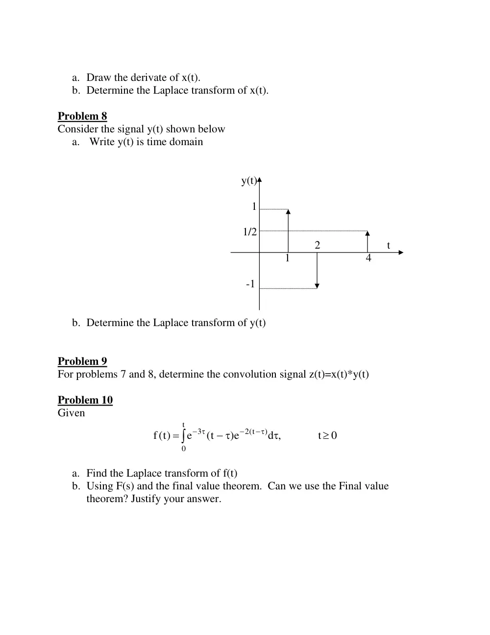Problem 8 Consider the signal y(t) shown below a. Write y(t) is time domain y(t) 1 1/2 2 t 1 4 -1 b. Determine the Laplace transform of y(t) Problem 9 For problems 7 and 8, determine the convolution signal z(t)=x(t)*y(t) Problem 10 Given           t 0 ) 2 t( 3 0 t d , e) t( e )t( f a. Find the Laplace transform of f(t) b. Using F(s) and the final value theorem. Can we use the Final value theorem? Justify your answer. 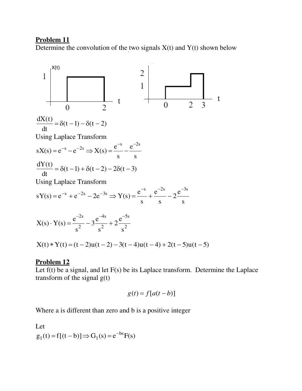Problem 11 Determine the convolution of the two signals X(t) and Y(t) shown below 2) t( )1 t( dt dX )t(       Using Laplace Transform s e s e X )s( e e )s( sX 2s s 2s s          )3 t( 2 2) t( )1 t( dt dY )t(          Using Laplace Transform s 2e s e s e Y )s( 2e e e )s( sY 3s 2s s 3s 2s s              2 s 5 2 s 4 2 s 2 s e 2 s e 3 s e Y )s( )s( X        5) 5)u t( 2 t( 4) 4)u t( t(3 2) 2)u t( t( Y )t( X )t(           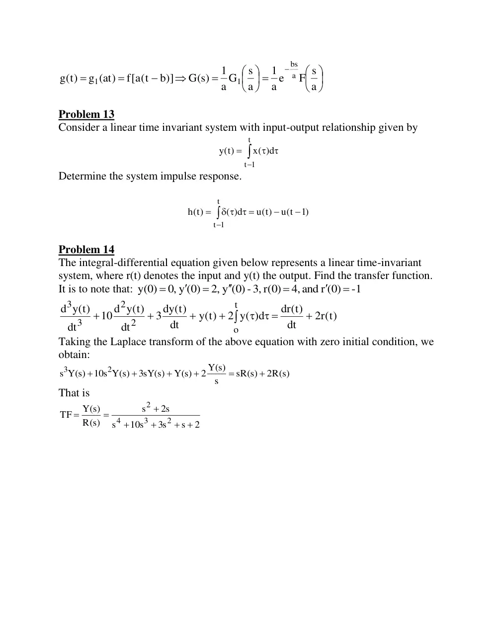Problem 12 Let f(t) be a signal, and let F(s) be its Laplace transform. Determine the Laplace transform of the signal g(t) )] [ ( ( ) b f a t g t   Where a is different than zero and b is a positive integer Let F )s( e )s( G b)] f[(t )t( g bs 1 1      X(t)                a F s a e 1 a s a G 1 G )s( b)] t( a[f g (at) )t( g a bs 1 1 Problem 13 Consider a linear time invariant system with input-output relationship given by      t 1 t x( )d y )t( Determine the system impulse response. )1 u t( u )t( ( )d )t( h t 1 t          Problem 14 The integral-differential equation given below represents a linear time-invariant system, where r(t) denotes the input and y(t) the output. Find the transfer function. It is to note that: -1 4, and r (0) (0) -3, r(0) 2, y (0) y ,0 y(0)        )t(r 2 dt dr )t( 2 y( )d y )t( dt dy )t( 3 dt d y )t( 10 dt d y )t( t o 2 2 3 3          Taking the Laplace transform of the above equation with zero initial condition, we obtain: 2R )s( sR )s( s 2 Y )s( Y )s( 3sY )s( 10s Y )s( s Y )s( 2 3       That is 2 s 3s 10s s 2s s )s( R Y )s( TF 2 3 4 2       