EECE 340 Homework Solution to Problem Set 1, Summer 2011

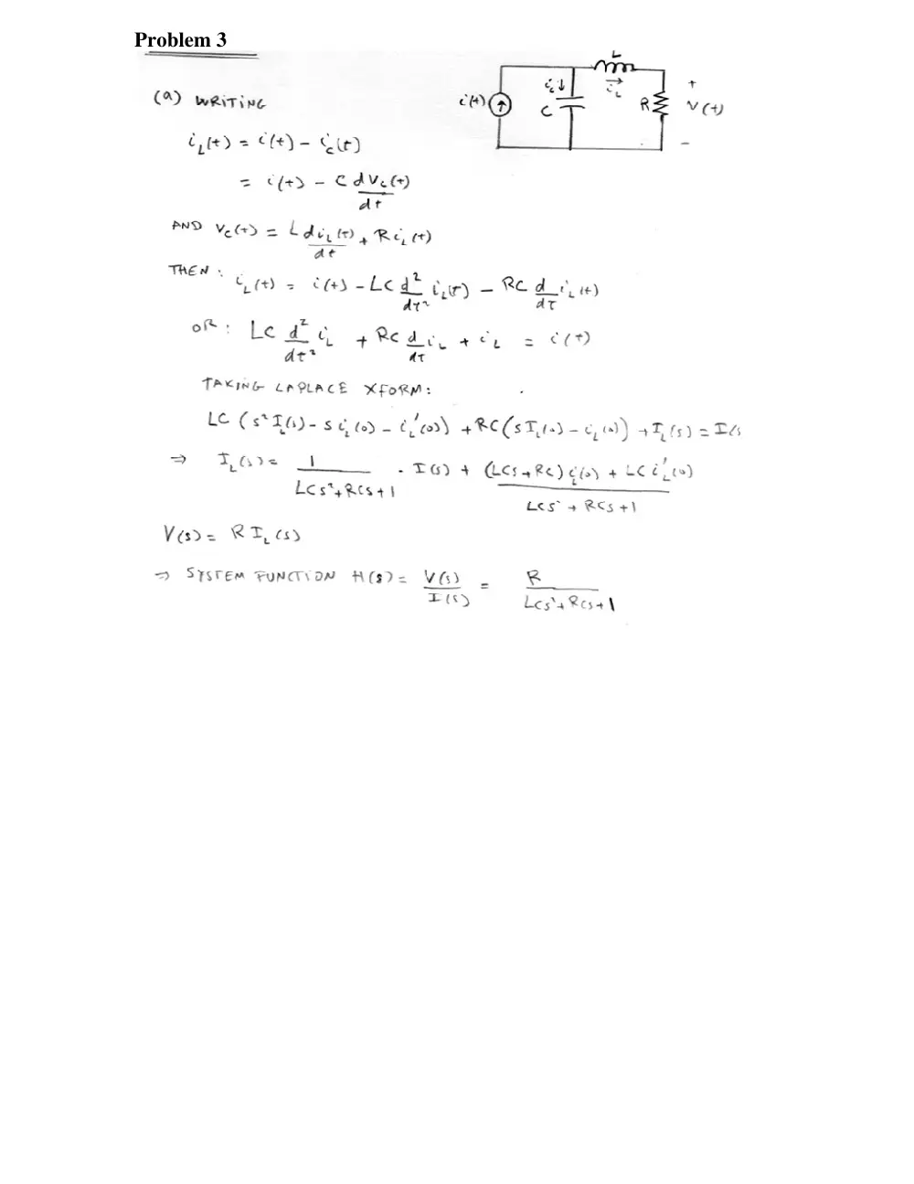
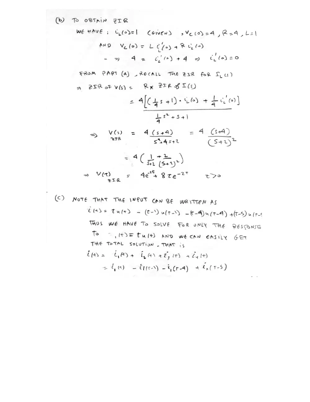
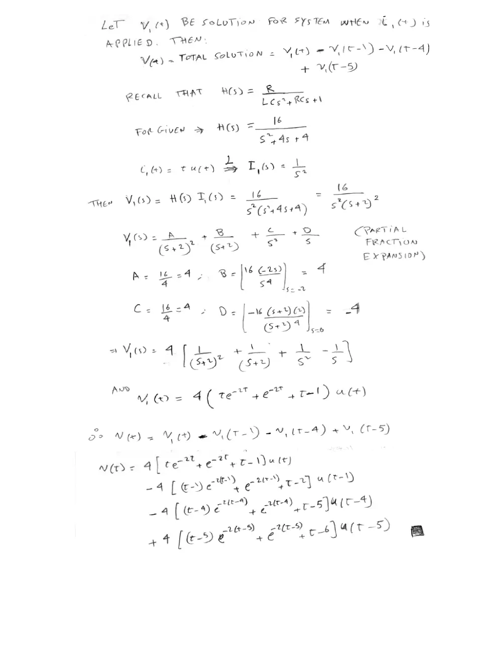
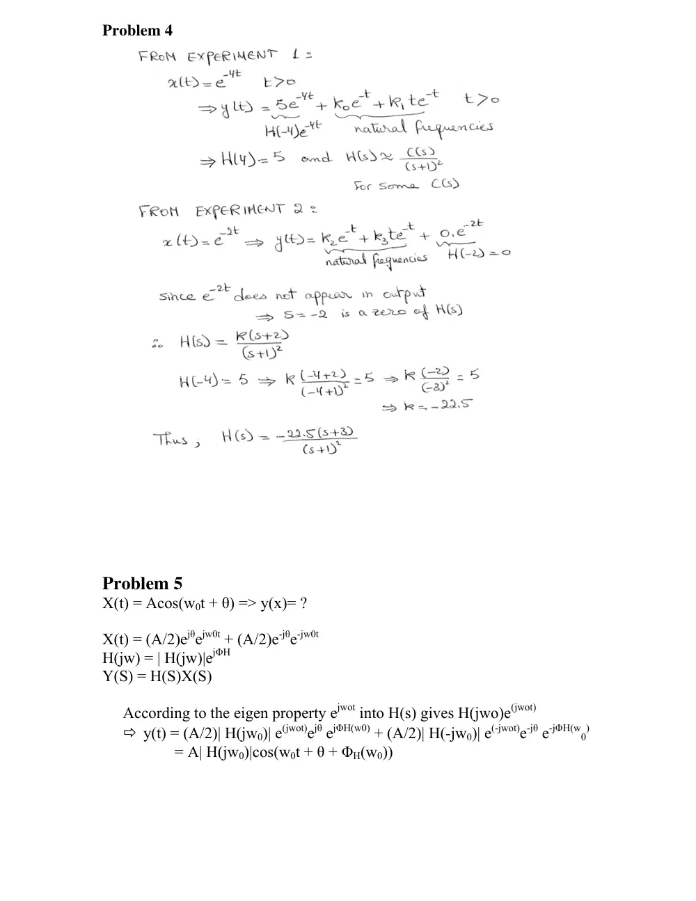
AMERICAN UNIVERSITY OF BEIRUT Department of Electrical and Computer Engineering EECE340- Spring 2011 Prof. Karameh Problem 1 Problem 2 Problem 3 Problem 4 Problem 5 X(t) = Acos(w0t + θ) => y(x)= ? 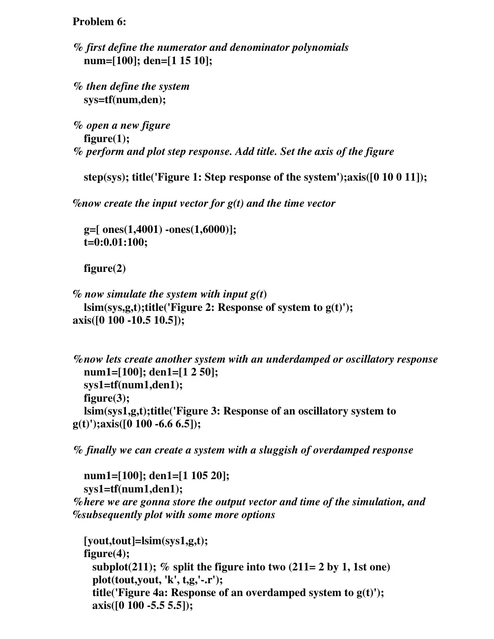X(t) = (A/2)ejθejw0t + (A/2)e-jθe-jw0t H(jw) = | H(jw)|ejΦH Y(S) = H(S)X(S) According to the eigen property ejwot into H(s) gives H(jwo)e(jwot) � y(t) = (A/2)| H(jw0)| e(jwot)ejθ ejΦH(w0) + (A/2)| H(-jw0)| e(-jwot)e-jθ e-jΦH(w 0 ) = A| H(jw0)|cos(w0t + θ + ΦH(w0)) Problem 6: % first define the numerator and denominator polynomials num=[100]; den=[1 15 10]; % then define the system sys=tf(num,den); % open a new figure figure(1); % perform and plot step response. Add title. Set the axis of the figure step(sys); title('Figure 1: Step response of the system');axis([0 10 0 11]); %now create the input vector for g(t) and the time vector g=[ ones(1,4001) -ones(1,6000)]; t=0:0.01:100; figure(2) % now simulate the system with input g(t) lsim(sys,g,t);title('Figure 2: Response of system to g(t)'); axis([0 100 -10.5 10.5]); %now lets create another system with an underdamped or oscillatory response num1=[100]; den1=[1 2 50]; sys1=tf(num1,den1); figure(3); lsim(sys1,g,t);title('Figure 3: Response of an oscillatory system to g(t)');axis([0 100 -6.6 6.5]); % finally we can create a system with a sluggish of overdamped response num1=[100]; den1=[1 105 20]; sys1=tf(num1,den1); %here we are gonna store the output vector and time of the simulation, and %subsequently plot with some more options [yout,tout]=lsim(sys1,g,t); figure(4); subplot(211); % split the figure into two (211= 2 by 1, 1st one) plot(tout,yout, 'k', t,g,'-.r'); title('Figure 4a: Response of an overdamped system to g(t)'); axis([0 100 -5.5 5.5]); [ystep,tstep]=step(sys1); subplot(212); plot(tstep,ystep); title('Figure 4b: Step Response of an overdamped system '); axis([0 30 0 5.5]); % add some more info to the last plot xlabel('time (sec)'); ylabel('y(t)'); OUTPUT: