PHYS 210L Lab Experiments, Spring 2008

Physics 210L ATWOOD’S MACHINEAND MOTION ON AN INCLINE 1. Object: The purpose of this experiment is to study the relationship between force, mass and acceleration using an Atwood’s machine apparatus. 2. Equipment: Science workshop interface, PC, Smart pulley, mass set and hanger, Air-track, glider, photogate timer and accessory photogate. 3. Theory: a) Atwood machine: The acceleration of an object depends on the net applied force and the mass. In an Atwood’s machine, the difference in weight between two hanging masses determines the net force acting on the system of both masses. The heavier mass is accelerated downward, and the lighter mass is accelerated upward. 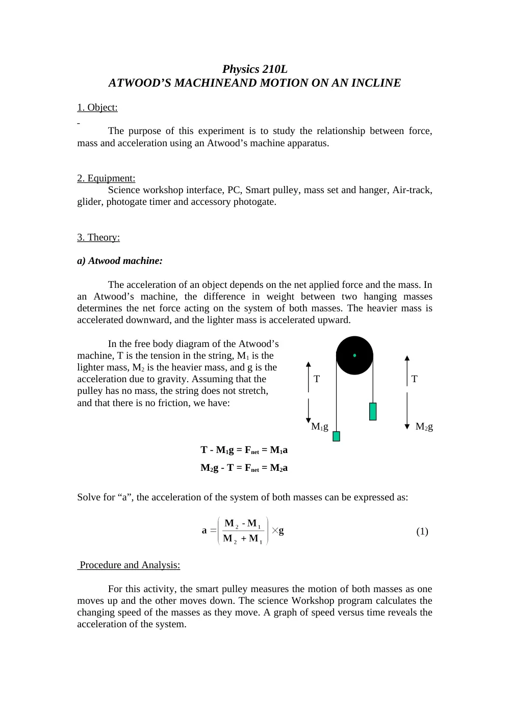In the free body diagram of the Atwood’s machine, T is the tension in the string, M1 is the lighter mass, M2 is the heavier mass, and g is the acceleration due to gravity. Assuming that the T T pulley has no mass, the string does not stretch, and that there is no friction, we have: M1g M2g T - M1g = Fnet = M1a M2g - T = Fnet = M2a Solve for “a”, the acceleration of the system of both masses can be expressed as: (1) Procedure and Analysis: For this activity, the smart pulley measures the motion of both masses as one moves up and the other moves down. The science Workshop program calculates the changing speed of the masses as they move. A graph of speed versus time reveals the acceleration of the system. 1. Connect the Science Workshop interface to the computer, turn on the interface, and turn on the computer. 2. Connect the stereo phone plug of the smart pulley to Digital Channel 1 on the interface. 3. Open the file titled P13_ATWD.SWS, found in the hard disk c:/. The document opens with a graph display of Velocity (m/s) versus time. 4. Enter the sampling options menu and setup the time (about 1.5 seconds) as a stop condition. i.e. the program will stop collecting data after 1.5 seconds of each trial. Click twice on the time axis and set the minimum value of time to zero and the maximum value to 2 seconds. Do the same for y-axis and set the minimum value of V to zero and the maximum value to 2 m/s. 5. Place two masses of M1 = 45 grams and M2 = 55 grams on both sides of the mass hanger as shown in Fig. 1. Move the heavier of the two masses upward to the highest position before it touches the pulley. Hold the system at this position. 6. When you are ready to begin the experiment, click the REC button to begin recording data, at the same time release the system from rest. 7. Run # 1 will appear in the data list in the experiment setup window. Using the plot V (m/s) versus time determine the acceleration of the system. 8. Change M1 and M2 in such a way that the net force is changed but the total mass remains the same. For example (M1 = 40 grams, M2 = 60 grams) then (M1 = 35 g, M2 = 65g) etc….. 9. Record your values in a table and compare your experimental acceleration with the calculated acceleration using Eq. 1. 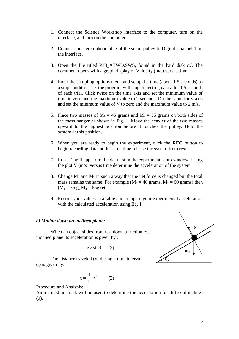b) Motion down an inclined plane: When an object slides from rest down a frictionless inclined plane its acceleration is given by : a = gsin (2) The distance traveled (x) during a time interval (t) is given by: x = (3) Procedure and Analysis: An inclined air-track will be used to determine the acceleration for different inclines (). 2  N mg  1. Using a block of wood incline the air track by an angle . Measure sin= Y/L. For best accuracy you should measure the thickness of the block using vernier calipers. 2. Place the photogate timer and the accessory photogate at about 50 cm apart. Turn on the photogate and set it at pulse. 3. Release the glider from rest down the incline and record the distance between the two photogates which is the distance the glider moves on the air track from where it first triggers the first photogate to where it first triggers the second photogate. Record the time that takes the glider to move this distance. Using Eq. 3 determine the value of a. (You shall repeat three times and then take the average value). 4. Repeat the same procedure for three different inclines. Plot the acceleration a (in m/sversus sin and using linear regression deduce the value of g along with its rms error. 5. Compare your value with the value found in the literature g = 9.8 m/s2. Comment. 3 BOYLE’S LAW Object: To study the relationship between pressure and volume for two different gases. Equipment: Science workshop interface; Personal Computer; Pressure, temperature and volume sensors; Syringe; PASCO Boyle’s law apparatus. 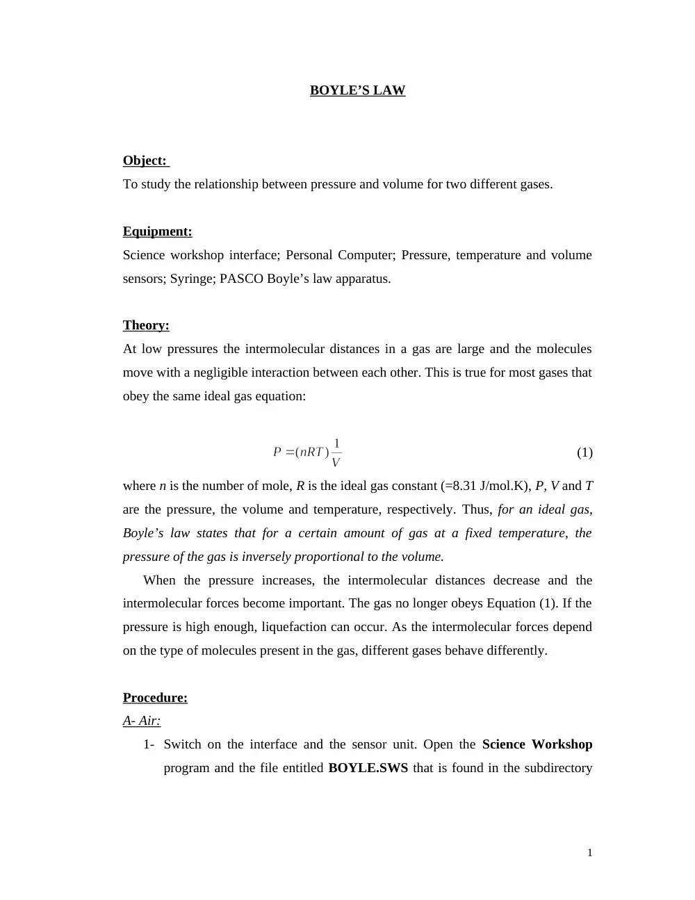Theory: At low pressures the intermolecular distances in a gas are large and the molecules move with a negligible interaction between each other. This is true for most gases that obey the same ideal gas equation: (1) where n is the number of mole, R is the ideal gas constant (=8.31 J/mol.K), P, V and T are the pressure, the volume and temperature, respectively. Thus, for an ideal gas, Boyle’s law states that for a certain amount of gas at a fixed temperature, the pressure of the gas is inversely proportional to the volume. When the pressure increases, the intermolecular distances decrease and the intermolecular forces become important. The gas no longer obeys Equation (1). If the pressure is high enough, liquefaction can occur. As the intermolecular forces depend on the type of molecules present in the gas, different gases behave differently. Procedure: A- Air: 1- Switch on the interface and the sensor unit. Open the Science Workshop program and the file entitled BOYLE.SWS that is found in the subdirectory 1 c:/Phys206. Take few minutes to study the windows that appear on your screen. 2- Make sure that the three analog Channels A, B and C correspond to the Pressure sensor (absolute), Voltage sensor and Temperature sensor, respectively. (These sensors are directly connected to the cylinder and are described on the next page, see Note 1). 3- With the valves open, pull the piston up to its highest value. Close the two gas valves. Your piston is now filled with air at atmospheric pressure. 4- Click the REC button to begin recording data. The Keyboard Sampling window opens. Push in the piston so that its height (h) in the cylinder is 16 cm. Wait for few seconds until the pressure reading stabilizes and type 16 as a value for the volume (see Note 2 on the next page). Click Enter to record your value of the pressure. 5- Repeat the procedure for h =15, 14, 13,…..,7 cm. These values will be automatically reported in a table and on a graph on your computer screen. After entering all these values, click the Stop Sampling button. 6- Plot the pressure P (atmosphere) versus 1/V (liters). From your graph deduce how many moles of air your cylinder contains. B. Butane gas: 1- To ensure you have as much butane gas in your cylinder, open both gas valves at the bottom of the cylinder and push the piston down to its lower limit. 2- Close one of the gas valves with the piston down. Introduce butane gas from the other valve to fill with cylinder to maximum volume and shut down the valve. Repeat this procedure a few times. 3- Repeat procedure “A.” with the butane gas that is now filling your cylinder. C. Estimation of the time interval for the temperature to become stable. 1- Fill your piston with air at atmospheric pressure and close the gas valves. 2- Drag the graph icon to the Temperature analog channel. Click on the sampling options button and then click on Keyboard to disable it. Also, in 2 the same window, switch the sampling rate to Fast and select of sampling rate of about 50 Hz. This option will enable the sensor to measure the temperature at periods of 0.02 seconds. Press OK. A graph will appear on your screen with time as the x-axis and Temperature as your y-axis. 3- Start recording the value of the temperature of the air in the cylinder by pressing on REC. 4- Push the piston down, in a single rapid shot, by about 3 cm and maintain it at this position while observing the variation of the temperature on the screen. 5- Release the piston when the temperature stabilizes and stop recording. 6- Observe the behavior of temperature with time for such a rapid compression of the gas. Estimate the time interval required for the temperature to stabilize (). What does this value represent? 7- Repeat this part of the experiment with Butane instead of air. 8- Close the Science Workshop program once you have finished the experiment. Do not save any of your data or files on the computer. Note 1: The volume sensor consists of a thin metallic sheet over which a voltage is applied. As the position of the piston is changed, the effective length of the sheet and consequently its resistance varies. This is detected as a change in voltage that is used to indicate the volume. The pressure sensor is based on a piezo-resistive material that is placed at the bottom of the cylinder. The electrical resistance of such a material changes as it is compressed and thus a change in pressure in the cylinder can be detected as a change in voltage across the material. The temperature sensor is the extremely fine nickel wire that is mounted at the base of the cylinder and whose resistivity strongly depends on its temperature. As the gas is compressed or expanded, the temperature of the gas and subsequently that of the wire change thus leading to a variation in the resistance of the wire. This effect is detected as a variation of the voltage across the wire that indicates changes in gas pressure. Note 2: The volume of the air is equal to the height × the area of the cylinder. The cylinder has an internal diameter Dint = 4.457 cm and the height of the piston can be read on the cylinder. 3 Bernoulli’s law. 1. Object: To experimentally verify Bernoulli’s law for fluid, and apply it to determine: (a) the air density and (b) the drag coefficient of a spherical object. 2. Equipment: Fan set with support, Venturi tube, precision manometer, pressure head, plastic tubes, and a plastic ball. 3. Theory: The total energy at any point in a liquid in motion may be separated into three different kinds of energy. (a) Potential energy, due to the elevation H of the liquid above some reference point, it is given by gH. (b) Pressure energy due to the pressure P at the point in question, this is given by P/ρ where ρ is the fluid’s density. (c) finally there’s the Kinetic energy expressed as V2/2 . This makes the total energy per unit mass of a flowing liquid: gh + p/ρ + v2/2. (1) Since energy is conserved, then the total energy of a flowing fluid will remain unchanged from one point to another. This is known as Bernoulli’s law formulated as: Gh1 + P1/ρ + V1 2/2 = Gh2 + P2/ρ + V1 2/2. (2) From Bernoulli’s equation we can get the air velocity (or the velocity of any fluid). If the fluid flow is horizontal, then H1 = H2. Therefore the original Bernoulli equation Gh1 + P1/ρ + V1 2/2 = Gh2 + P2/ρ + V2 2/2. Becomes P1/ρ + V1 2/2 = P2/ρ + V2 2/2. By measuring the pressure difference ΔP=P2-P1, we can determine the fluid velocity difference. V1 2 – V2 2 = (2/ ρ).( P2-P1) If we’re measuring the air velocity, and we want a value with respect to the surrounding still atmosphere, then: V2 = 0 & ΔP=P2-P1 where P2 is the atmospheric pressure. Therefore the expression becomes: V2 = (2/ρ).ΔP (3) Another basic principle related to fluid in motion is the continuity principle, this simply states that the volume of fluid entering a tube is equal to the volume of fluid leaving it (actually this is only true for incompressible fluids, but it is applicable to air at relatively low velocities), this is expressed by: R= A1V1 = A2V2. (4) Where A1 and A2 are the cross section area at different points of the tube, V1 and V2 are the fluid velocity at point 1 and 2 respectively, and R is the flow rate in m3/s. 4. Procedure: A) Drag coefficient. 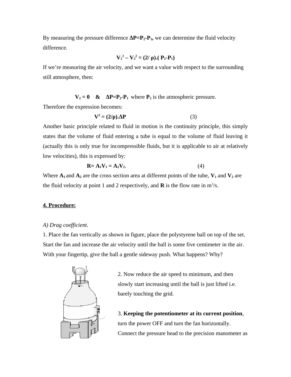1. Place the fan vertically as shown in figure, place the polystyrene ball on top of the set. Start the fan and increase the air velocity until the ball is some five centimeter in the air. With your fingertip, give the ball a gentle sideway push. What happens? Why? 2. Now reduce the air speed to minimum, and then slowly start increasing until the ball is just lifted i.e. barely touching the grid. 3. Keeping the potentiometer at its current position, turn the power OFF and turn the fan horizontally. Connect the pressure head to the precision manometer as shown in figure below. Make sure the high pressure end is connected to the tube having its intake perpendicular to the air flow. 4. Turn the power ON, and hold the pressure head no more than 10 cm away from the fan nozzle, record the air velocity. 5. If the force due to air resistance is equal to F = Cw.V2.A.ρ/2 where Cw is known as the drag coefficient and depends on the shape of the body in question, ρ is the air density (1.3 Kg/m3), V the air velocity, and A the area of the ball. Try to determine the drag coefficient using the air velocity you just got. Hint: since the ball is just lifted above the fan the force due to air resistance should be equal to the weight. B) Flow rate. 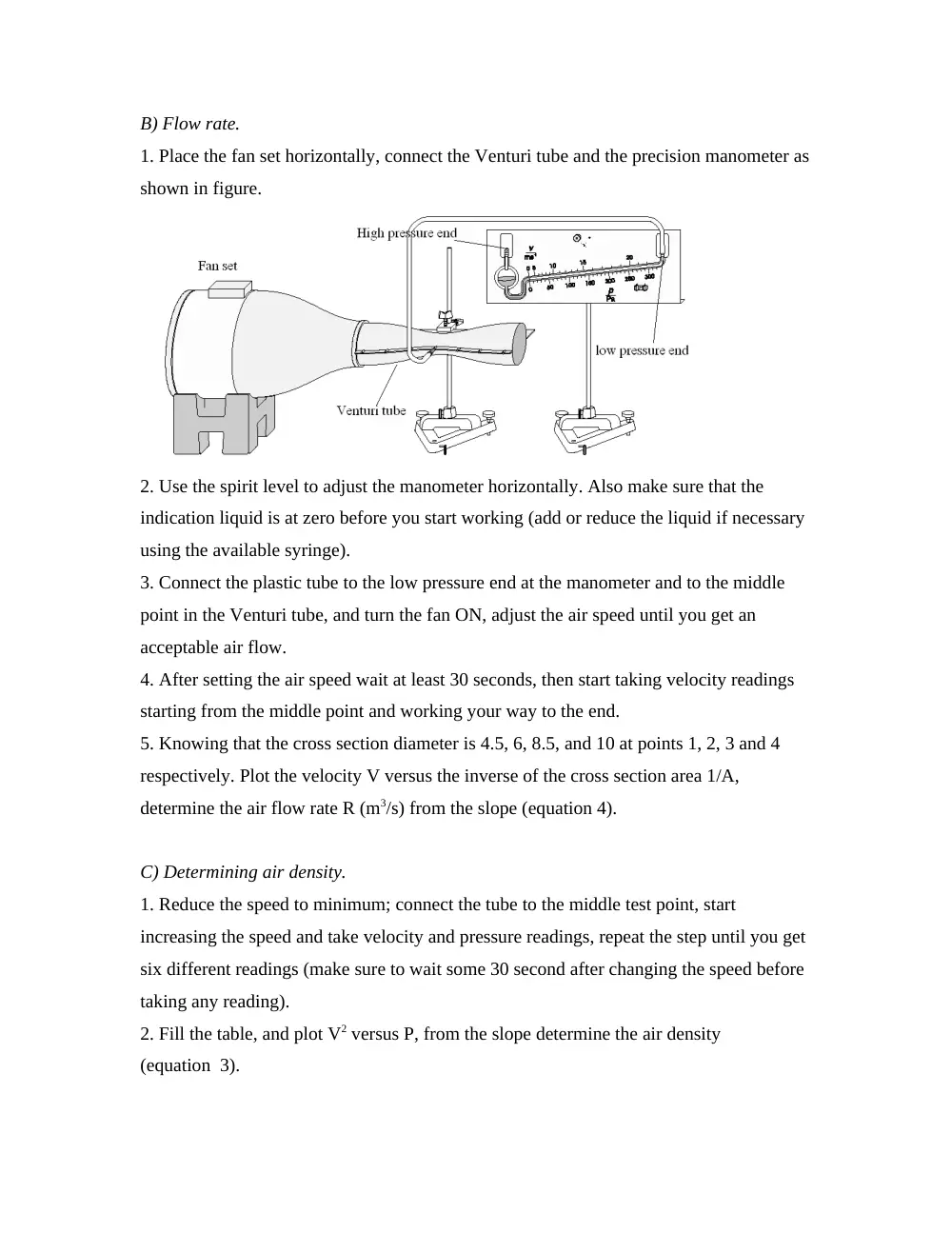1. Place the fan set horizontally, connect the Venturi tube and the precision manometer as shown in figure. 2. Use the spirit level to adjust the manometer horizontally. Also make sure that the indication liquid is at zero before you start working (add or reduce the liquid if necessary using the available syringe). 3. Connect the plastic tube to the low pressure end at the manometer and to the middle point in the Venturi tube, and turn the fan ON, adjust the air speed until you get an acceptable air flow. 4. After setting the air speed wait at least 30 seconds, then start taking velocity readings starting from the middle point and working your way to the end. 5. Knowing that the cross section diameter is 4.5, 6, 8.5, and 10 at points 1, 2, 3 and 4 respectively. Plot the velocity V versus the inverse of the cross section area 1/A, determine the air flow rate R (m3/s) from the slope (equation 4). C) Determining air density. 1. Reduce the speed to minimum; connect the tube to the middle test point, start increasing the speed and take velocity and pressure readings, repeat the step until you get six different readings (make sure to wait some 30 second after changing the speed before taking any reading). 2. Fill the table, and plot V2 versus P, from the slope determine the air density (equation 3). GEOMETRICAL OPTICS: LAW OF REFRACTION Object: To study refraction and total internal reflection using Snell’s law. Equipment: Ray box (white and colored rays); Rhombus; Protractor; White paper; Convex lens. Theory: When a ray of light crosses the interface separating two media of different index of refraction n1 and n2, the ray is subject to a refraction following Snell’s law, (1) where is the angle of incidence and is the angle of refraction as shown in Fig.1. If a ray of light is traveling from a medium of lesser index of refraction is incident with an angle greater than the “critical angle”, c, there is no refracted ray and total internal reflection occurs (See Fig. 2). If the angle of incidence is exactly the critical angle, the angle of the refracted ray is 90o. In this case, using Snell’s law, we can deduce that assuming that the medium of lesser index of refraction is air with n2=1 and the medium of greater refraction is n1=n. Light rays originating from the bottom surface of a block of material refract at the top surface as the rays emerge from the material into the air, as represented in Fig.3. When viewed from above, the apparent depth, a, of the bottom surface is less than the actual thickness, t, of the block. The apparent depth is given by d=t/n where n is the index of refraction of the material. 1 Procedure: A- Snell’s law: 1- Place the ray box, label side up, on a white sheet of paper on the table. Slide the ray mask until only one white ray is showing. 2- Place the Rhombus on the table and position it so the ray passes through the parallel sides as shown in Fig. 4. 3- Mark the position of the parallel surfaces of the rhombus and trace the incident and transmitted rays. Mark carefully where the ray enters and leaves the rhombus. 4- Remove the rhombus and draw, on the paper, a line connecting the points where the rays enters and leaves the rhombus. Also draw the normal to the two parallel surfaces of the rhombus. 5- Measure, from the normal, the angle of incidence  and the angle of refraction with a protractor. 6- Repeat the experiment for four other angles of incidence and plot sinversus sin. Deduce the index of refraction of the rhombus from your curve. B- Total internal reflection: 1- Position the rhombus as shown in Fig.5 and rotate it until the emerging ray just barely disappears (Just as it disappears, the ray separates into colors, the rhombus is correctly positioned if the red has just disappeared). 2- Mark the surfaces of the rhombus, the exact point where the ray is internally reflected as well as the entrance and exit point of the ray. 3- Remove the rhombus and draw the rays that are incident upon and reflected off the inside surface of the rhombus, as shown in Fig. 6. Measure the total angle between these rays. Show that this angle is equal to 2c. 4- Deduce the index of refraction of the rhombus from these measurements. How does your value compared to the one determined in Part A? 2 C- Apparent Depth: 1- Place the ray box on a white sheet of paper and slide the mask on the mask box so that five parallel white rays are produced. Use a screen to block the three middle rays, leaving only the outside two rays. 2- Place the convex lens in front of the ray box and mark the place where the two rays cross each other. 3- Place the rhombus as shown in Fig.7. The bottom surface of the rhombus must be exactly at the point where the two rays cross. 4- Trace the bottom and top surfaces of the rhombus and trace the rays diverging from the top surface. 5- Remove the rhombus, turn off the light source and trace the diverging rays back into the rhombus. The place where the two rays cross (inside the rhombus) is the apparent position of the bottom of the rhombus when viewed from the top. 6- Measure the apparent depth, d, and the thickness of the rhombus, t. Determine from these measurements the index of refraction of the rhombus. How does your values compare to those measured in Parts A and B? 3 4 GEOMETRICAL OPTICS II: MIRRORS AND LENSES Object: To measure the focal distances of convex and concave mirrors as well as converging and diverging lenses. Equipment: Ray box (white and colored rays); Curved mirrors; Protractor; White paper; Convex and concave lenses. Theory: A concave cylindrical mirror will focus parallel rays of light at the focal point. The focal length is the distance from the focal point to the center of the mirror surface. A convex mirror also has a focal point. If parallel rays are incident on a convex mirror, the reflected rays seem to come from a single point, the focal point, behind the mirror. For both the concave and convex mirrors, the radius of curvature of the mirror is twice its focal length. Parallel rays of light passing through a thin convex (converging) lens cross at the focal point of the lens. A thin concave (diverging) lens causes incident parallel rays to diverge after exiting the lens. Those diverging rays seem to originate from one single point before the lens, the focal point. For both types of lenses, the focal length is measured from the center of the lens to the focal point. The lensmaker’s equation can be used to calculate the focal length of a lens and its is given by (Eq. 1) where f is the focal length, n is the relative index of refraction of the lens material and R1 and R2 are the radii of curvature of the lens surfaces. In this notation, R is positive for a convex surface (as viewed from outside the lens) and R is negative for a concave surface. 1 Procedure: A- Concave and Convex Mirrors: 1- Place the ray box, label side up, on a white sheet of paper on the table. Slide the ray mask until five parallel white rays are emitted. 2- Shine the rays straight into the concave mirror so the light is reflected back towards the ray box. . 3- Draw the surface of the mirror and trace the incident and reflected rays. The place where the five reflected rays cross each other is the focal point of the mirror. Measure the focal length from the center of the concave mirror surface to the focal point. 4- Measure the radius of curvature of the mirror and deduce from your measurement the value of the focal length. How does it compare to the one that you have in Step3. 5- Repeat Steps 1 through 3 for the convex mirror. In this case, the reflected rays are diverging for a convex mirror and they will not cross. Use a ruler to extend the reflected rays back behind the mirror’s surface. The focal point is where these extended rays cross. B- Concave and Convex Lenses: 1- Place the ray box on a white sheet of paper. Using the five white rays from the box, shine the rays straight into the convex lens. Trace around the surface of the lens and trace the incident and transmitted rays. 2- Determine the focal length of the lens. 3- Repeat Steps 1 and 2 for the convex lens. 4- Place the convex lens in the path of the five rays. Block out the center three rays and mark the focal point of the outer two rays. Slide the mask to the position that gives three rays and mark the focal point for the inner three rays. Are the focal points the same? 2 C- Lensmaker’s equation (Concave lens): 1- To determine the radius of curvature, put the concave lens back in the path of the rays and observe the faint reflected rays off the first surface of the lens. The front lens can be treated as a concave mirror having a radius of curvature equal to twice the focal length of the mirror. 2- Trace the surface of the lens and the incident rays and the faint reflected rays. Measure the distance from the center of the front curved surface to the point where the faint rays cross. The radius of curvature of the surface is twice this distance. Record the radius of curvature. 3- Use the lensmaker’s formula to calculate the index of refraction of the material from which the lens is made of. 3 INTERFERENCE AND DIFFRACTION 1. Object: To investigate the double slit interference and single slit diffraction phenomena. 2. Equipment: Diode laser; single and double slit disks and screen. . 3. Theory: a- Diffraction: In this part of the experiment, the interference of waves originating from different point sources within a single slit is studied. This phenomenon is called diffraction and occurs when the width of the slit is larger than the wavelength of the light beam. The set- up used for studying diffraction is shown in Fig.1. The laser illuminates a single slit of width w (w. Wavelets that are originated from different points within the slit can interfere constructively or destructively. This leads to the formation of a diffraction pattern that consists of a succession of dark and bright fringes observed on a screen placed at a distance D from the slit. 1 Laser Beam w D Screen P Slide with single slit Diffraction pattern  Y Figure 1- Experimental set-up used for the study of the diffraction of light waves. It can be shown that the condition for obtaining dark fringes is given by sin= m(/w) m=1, 2, 3… (1) where we have considered that rays originating from each point source within the slit make the same angle  with the horizontal because w<<D. The integer m is called the order of the fringe. If the angle  is very small (<0.1 rad), Eq.(1) becomes  = m(/w) (2) On the screen, the separation Y between the mth dark fringe and the central bright fringe is given by Y = (mD)/w (3) b- Interference: In this part of the experiment, the interference of light emitted by two similar light sources is studied using the set-up depicted in Figure 2. A diode laser beam is incident on a pair of slits S1 and S2, separated by a distance d. The slits act as two light sources whose waves can interfere with each other. This leads to the formation of a variable intensity pattern that can be observed on a screen placed at a distance D from the slits with D>>d. Dark and bright fringes on the screen indicate regions of minimum and maximum light intensity that respectively correspond to destructive and constructive interference. Figure 2- Set-up used for the study of the interference of two light waves. 2 Laser Beam   l l d  l S S1 2 D Screen P Slide 1 2 Interference pattern X The light waves from slits S1 and S2 interfere constructively or destructively at a certain point P on the screen depending on the difference l between l1 and l2, l1 and l2 being respectively the distance from S1 and S2 to P. It can be shown that l = l1-l2 = d sin whereby we have considered that S1P and S2P make the same angle  with the horizontal since d<<D. When l = m (m being an integer), constructive interference occurs so that bright fringes are obtained for sin = m(/d) m = 0,1, 2, 3… (5) The value of m is called the order of the fringe. If the angle  is very small (<0.1 rad), then sin= tan=  so that  = m(/d) (6) On the screen, the separation, X, between two adjacent bright fringes is given by X = (D)/d (7) It can be shown that this is also equal to the separation between adjacent dark fringes. 4. Procedure & Analysis: a- Diffraction:. (1) Switch on the laser and place the single slit disk at a distance of about 3 cm. Align the laser so that it is incident on the 0.04 mm slit and a diffraction pattern is seen on the screen. (2) Determine the distance from the slit to the screen and measure the separation between the two dark fringes on the opposite side of the central maximum. (3) Estimate the beam by using Eq.(3). Repeat the procedure for different slits. Estimate the average wavelength of the laser. b- Interference: (1) Turn on the laser and place the double slit disk (slit width =0.04 mm and separation = 0.25 mm) in such a way that both slits are irradiated by the laser. A pattern of fringes should be seen on the screen. (2) Take several measurements of X, the separation between two adjacent bright fringes. Repeat for different double slits and measure D. 3 (3) Determine from your measurements the value of . Comment. 4 VII. MICHELSON INTERFEROMETER 1. Objective : To measure the wavelength  of a Helium-Neon Laser and the refractive index of air using a Michelson interferometer . 2. Equipment : Michelson interferometer, He-Ne laser, Vacum pump, Cell with glass Windows, Vernier caliper, balloon and lighter fuel gas. 3. Theory: The Michelson interferometer is an instrument in which a light beam is split into two beams, which after traveling along different paths are reunited and allowed to interfere (figure1) Fig. 1: Shematic view of Michelson Interferometer setup. M2 S M1 M Cell L To Eye MM1 = d1 MM2 = d2 P American University of Beirut, Physics Department. Phys210 L. ___________________________________________________________________________________ A source of monochromatic light transmits a beam of light to half-silvered mirror M (beam-splitter). About half of the incident light is reflected to mirror M1, the rest of the light is transmitted to mirror M2. The reflected light from M1 passes through the beam-splitter M and arrives to P. The reflected light from M2 falls on the beam-splitter and is reflected towards P. Both beams are therefore brought at the beam-splitter, resulting interference. Thus at P an interference pattern will be observed. The interference pattern is a set of concentric circular fringes of alternating intensity (dark and bright). The central spot is due to that part of the beam that is incident normally to the mirrors M1 and M2. Other parts of the beam that are not incident normally to the mirrors travel different paths and the nature of the interference varies from point to point, depending on the angle of incidence. If the path difference is a multiple of wavelength  of the light, then a bright fringe will be observed. In the case that the path difference is an odd multiple of /2, a dark fringe results. Because of the cylindrical symmetry of the light beam the fringes will be circular. When the mirrors are not exactly perpendicular to each other, one observes curved fringes that are part of circular fringes. If the circles are large enough, the fringes appear to be straight. The optical path difference between the two beams for the central spot is: X0 = 2d2 –2d1 (1) This path difference determines the nature of the interference, and if it were to change then the interference conditions would change and the interference would pass from one state to another. The Michelson interferrometer can accommodate a copper cell with glass windows that can evacuated then slowly filled with a choosen gas. When the cell is inserted in the path of the second beam, the optical path difference becomes: X = X0 +2L (nx – nAir) (2) Where L is the length of the cell and nx is the index of refraction of the gas contained in the cell. When the cell is evacuated the index of refraction nx is exactly 1, but otherwise depends on the gas and the pressure in the cell. One starts with an evacuated cell so that Xi = X0 + 2L(1-nAir) (3) 2 American University of Beirut, Physics Department. Phys210 L. ___________________________________________________________________________________ and slowly introduces the gas whose index of refraction is to be measured into the cell. As the gas is slowly introduced in the cell, nx changes slowly and therefore the optical path difference changes. The interference at every point alternates between destructives and constructive, and the fringes appear to move. Every time a bright fringe passes by a certain point, the interference at that point will have gone through a cycle of constructive, destructive and back to constructive. The optical path will have changed by one