EECE 210 Lecture 4, Fall 2014

Chapter 4 Circuit Theorems Objective and Overview The Chapter presents some theorems that apply to electric circuits, and which center primarily around Thevenin’s theorem. Thevenin’s theorem takes circuit equivalence to its extreme, by representing any LTI circuit, between any two given terminals, by a linear-output voltage source in the case of resistive circuits. Thevenin’s theorem is arguably the most important theorem in circuit analysis, both from theoretical and practical viewpoints. It is therefore discussed at length with several examples that highlight some of its aspects. The discussion of Thevenin’s equivalent circuit is naturally followed by a discussion of its current-source counterpart, namely, Norton’s equivalent circuit. Norton’s equivalent circuit has the added significance that some circuits may have a Norton’s equivalent circuit, but not a Thevenin’s equivalent circuit, just as the converse is also true. The Chapter ends with the substitution theorem, which is a useful theorem that simplifies the analysis of some types of circuits, and which can be readily proved using Thevenin’s theorem. A particular form of the substitution theorem, the source absorption theorem, is presented as a useful tool for replacing dependent sources by resistors in some cases, which again simplifies circuit analysis in these cases. Discussion in this Chapter and in Chapters 5 and 6 is restricted to the dc state. 4.1 Excitation by Dependent Sources Before presenting Thevenin’s theorem, the following concept is discussed: Concept: Dependent sources alone do not excite a stable circuit. To illustrate this concept, consider the circuit of Figure 4.1.1. From KCL at the upper essential node, iY + 2IY = vX/6, or, vX = 18iY (4.1.1) From KVL around the mesh on the left, 3vX – 4iY – vX = 0, or, vX = 2iY (4.1.2) Substituting for iY from Equation 4.1.2 in Equation 4.1.1, vX = 9vX, or, 8vX = 0 (4.1.3) It follows that vX = 0, which also makes iY = 0. This material is copyrighted and must not be reproduced or distributed. 1-4 – + – + vX iY 3vX 2iY 4  6  Figure 4.1.1 Although demonstrated for a particular circuit, it is true in general that if dependent sources are the only sources in a circuit, the circuit is relaxed, that is, all voltages and currents in the circuit are zero. An exception is encountered in circuits with a strong enough positive feedback. These circuits are unstable in that their responses are unbounded, that is, their magnitudes increase with time until they are limited by some nonlinearity in the circuit. Such circuits are not of interest to us in this book. That is the reason for the ‘stable’ qualifier in the statement of the concept enunciated at the beginning of this section. Although they alone do not excite a circuit, dependent sources do, of course, affect the voltages and currents in the circuit. They can deliver or absorb energy, just like independent sources. It will be shown later (Section 5.1, Chapter 5) that dependent sources effectively modify the values of some resistances in the circuit. 4.2 Thevenin’s Theorem In the context of resistive circuits, Thevenin’s theorem can be stated as follows: Statement: A circuit consisting of ideal resistors and sources is equivalent, at a specified pair of terminals, to a linear-output voltage source. The equivalent circuit, consisting of an ideal voltage source in series with a resistor is known as Thevenin’s equivalent circuit (TEC). The open-circuit voltage is referred to as the Thevenin voltage, VTh, and the source resistance as the Thevenin resistance, RTh. The open-circuit voltage and source resistance were defined for a linear-output voltage source in Section 3.6, Chapter 3. Thevenin’s theorem takes circuit equivalence to the extreme, in that it reduces any LTI circuit at a given pair of terminals to the simplest possible n equivalent, namely an ideal voltage source in series with a resistor. 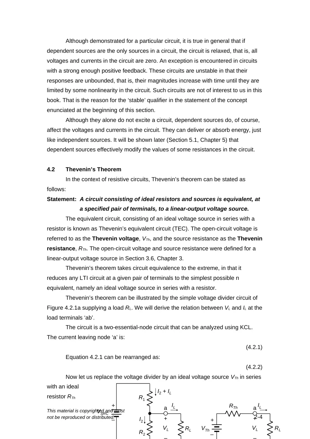Thevenin’s theorem can be illustrated by the simple voltage divider circuit of Figure 4.2.1a supplying a load RL. We will derive the relation between VL and IL at the load terminals ‘ab’. The circuit is a two-essential-node circuit that can be analyzed using KCL. The current leaving node ‘a’ is: (4.2.1) Equation 4.2.1 can be rearranged as: (4.2.2) Now let us replace the voltage divider by an ideal voltage source VTh in series with an ideal resistor RTh This material is copyrighted and must not be reproduced or distributed. 2-4 + – VSRC R1 – + VL I2 + IL I2 IL a R2 RL – + VL IL a RL + – VTh RTh (Figure 4.2.1b). KVL gives: (4.2.3) Equation 4.2.3 is of the same form as Equation 4.2.2, in accordance with Thevenin’s theorem. Moreover, the two equations become identical if VTh and RTh are given by: and (4.2.4) Under these conditions, VTh in series with RTh is equivalent to the voltage divider circuit at terminals ‘ab’, since they have the same VL-IL relation (Figure 4.2.1c). RTh is the source resistance, and VTh is the open-circuit voltage at terminals ‘ab’, when IL = 0. Although shown to apply for the voltage divider circuit, Thevenin’s theorem in fact applies to a circuit of any complexity consisting of ideal sources and resistors. Evidently, replacing a complex circuit by its TEC between a given pair of terminals greatly simplifies analysis of the overall circuit, as will be demonstrated on many occasions. Derivation of TEC In the preceding discussion VTh and RTh were determined by deriving the VL-IL relation at the given pair of terminals, which is unnecessarily complicated. A simpler procedure is suggested by the nature of TEC itself and the VL-IL relation. Since the plot of VL vs. IL is a straight line (Figure 4.2.1c), this line is uniquely determined by specifying its slope, whose magnitude is Rsrc, and a point through which the line passes, such as the intercept on the voltage axis. This intercept is VTh and equals VL, when IL = 0. It can, therefore, be determined directly from the circuit as the open- circuit voltage at terminals ‘ab’. Thus, if RL is removed from the circuit (Figure 4.2.2a), it follows from voltage division that: (4.2.5) which is the same as Equation 4.2.4. RTh can be determined in one of two ways: either directly, or as the ratio of the voltage intercept VTh in Figure 4.2.1c to the current intercept, which is the short-circuit current ISC. When terminals ‘ab’ are short-circuited (Figure 4.2.2b), it follows from Ohm’s law that: (4.2.6) This material is copyrighted and must not be reproduced or distributed. 3-4 + – VSRC R1 – + VTh I2 (a) (b) I2 IL = 0 a b R2 + – VSRC R1 ISC I2 = 0 a b R2 ISC Figure 4.2.2 Figure 4.2.3 (a) (b) IT a RTh + – VT b IT a RTh b + – VT The ratio VTh/ISC is, from Equations 4.2.5 and 4.2.6, R1R2/(R1 + R2), the same as the expression for RTh in Equation 4.2.4. The direct method of determining RTh is suggested by Figure 4.2.1b. If VTh is set to zero, that is, replaced by a short-circuit (Section 2.4, Chapter 2) and a test voltage source VT is applied between terminals ‘ab’, then RTh = VT/IT (Figure 4.2.3a). That is, RTh is Req seen by the test source between terminals ‘ab’. Alternatively, a test current source IT may be applied and RTh is again given by VT/IT (Figure 4.2.3b). But what does setting VTh to zero imply in the original circuit? It implies setting all independent sources to zero , for this removes excitation from the circuit and reduces all currents and voltages in the circuit to zero, including VTh. As mentioned in Section 4.1, dependent sources alone do not excite the circuit. Hence, VTh becomes zero when all independent sources are set to zero while leaving dependent sources unchanged. Note that although dependent sources alone do not excite the circuit, they do affect the relations between voltages and currents in the circuit in the presence of independent sources by effectively altering the values of resistances, including RTh . Setting dependent sources to zero will therefore alter RTh, whereas setting independent sources to zero removes excitation from the circuit, without altering RTh. Bear in mind that an ideal voltage source is set to zero by replacing it with a short circuit (Section 2.4, Chapter 2), and that an ideal current source is set to zero by replacing it with an open circuit (Section 2.5, Chapter 2), It should be noted that applying a test source to determine RTh, as in Figures 4.2.3a and b, is a formal and general method of determining Req between any two terminals of a circuit, with independent sources set to zero. That was, in fact, the method used for determining Reqs and Reqp in Chapter 3 (Figures 3.2.1 and 3.2.3). Using a test source is the only applicable method for determining Req in the presence of dependent sources. However, In the absence of dependent sources , Req, and hence RTh, can be determined more directly using series/parallel combinations of resistors, star-delta transformation, etc. The procedure for deriving TEC can be summarized as follows: 1. Determine VTh as the open-circuit voltage at the specified terminals. 2. Determine the short-circuit current ISC at the specified terminals, which gives RTh as VTh/ISC. 3. Set all independent sources in the given circuit to zero, leaving dependent This material is copyrighted and must not be reproduced or distributed. 4-4 sources unchanged. RTh is the resistance Req looking into the specified terminals. Formally, this resistance is obtained by applying a test voltage source or a test current source and determining Req as the ratio of the voltage at the source terminals to the source current. In the absence of dependent sources, Req can be derived directly from series/parallel combinations of resistors, and using star- delta transformations, if necessary. The following should be noted concerning this procedure: 1. Since VTh = RThISC, only two of the three quantities in this relation need be determined through the aforementioned three steps. However, it is useful for checking purposes to determine all three of these quantities independently. 2. Moreover, some of the aforementioned three steps many be easier to implement than others. Thus, setting independent sources to zero can make the circuit particularly simple. 3. In some cases, VTh = 0, which means that ISC = 0. It follows that VTh/ISC is 0/0, which is indeterminate. In this case, RTh can only be determined by Step 3 of the aforementioned procedure. This is illustrated by Example 4.2.3. 4. A potential ambiguity in deriving TEC at a pair of terminals is whether or not to include in TEC a resistor R that is connected between the given pair of terminals. The ambiguity is resolved in this book by the way the resistor is drawn with respect to the given terminals or by the way TEC is required. In Figure 4.2.4a, for example, R is drawn beyond the terminals at which TEC is required, as was done in Figure 4.2.1a. The implication is that R should not be included in TEC. Even without drawing the terminals in this manner, requiring “TEC seen by R”, or “TEC looking into terminals ‘ab’” means that R should not be included in TEC. On the other hand, if the given terminals are beyond ‘R’, as in Figure 4.2.4b, the implication is that R should be included in TEC. Requiring “TEC between terminals ‘ab’” is unambiguous in this case. 5. Even in the case of Figure 4.2.4b, it may be advantageous to remove R and determine an intermediate TEC from the simpler circuit that results when R is removed. After obtaining this TEC, R is connected to the terminals of this TEC and the final TEC derived. This procedure is illustrated by Example 4.2.4. This material is copyrighted and must not be reproduced or distributed. 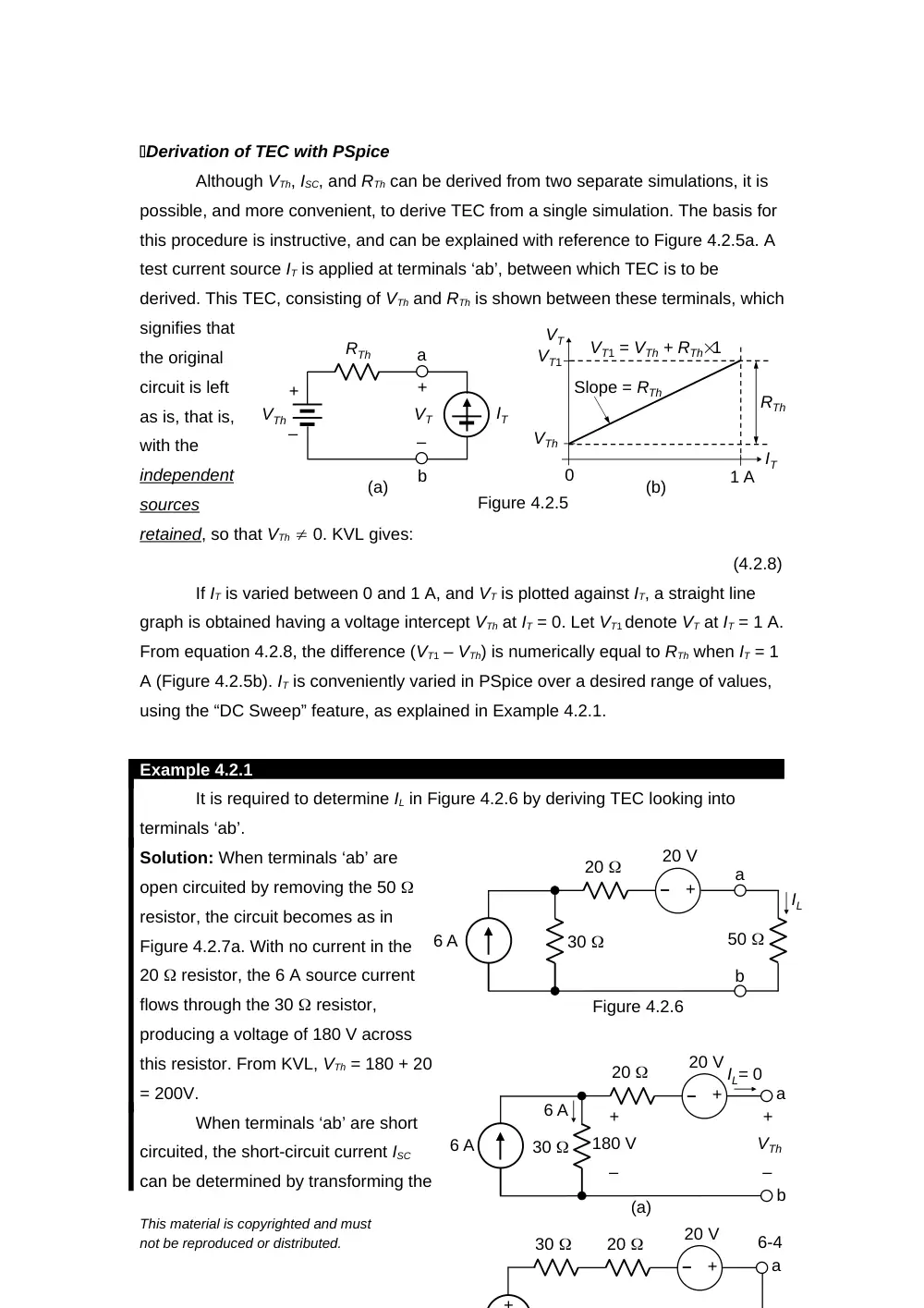5-4 a R b (a) (b) Figure 4.2.4 Circuit N a R b Circuit N Derivation of TEC with PSpice Although VTh, ISC, and RTh can be derived from two separate simulations, it is possible, and more convenient, to derive TEC from a single simulation. The basis for this procedure is instructive, and can be explained with reference to Figure 4.2.5a. A test current source IT is applied at terminals ‘ab’, between which TEC is to be derived. This TEC, consisting of VTh and RTh is shown between these terminals, which signifies that the original circuit is left as is, that is, with the independent sources retained, so that VTh  0. KVL gives: (4.2.8) If IT is varied between 0 and 1 A, and VT is plotted against IT, a straight line graph is obtained having a voltage intercept VTh at IT = 0. Let VT1 denote VT at IT = 1 A. From equation 4.2.8, the difference (VT1 – VTh) is numerically equal to RTh when IT = 1 A (Figure 4.2.5b). IT is conveniently varied in PSpice over a desired range of values, using the “DC Sweep” feature, as explained in Example 4.2.1. Example 4.2.1 It is required to determine IL in Figure 4.2.6 by deriving TEC looking into terminals ‘ab’. Solution: When terminals ‘ab’ are open circuited by removing the 50  resistor, the circuit becomes as in Figure 4.2.7a. With no current in the 20  resistor, the 6 A source current flows through the 30  resistor, producing a voltage of 180 V across this resistor. From KVL, VTh = 180 + 20 = 200V. When terminals ‘ab’ are short circuited, the short-circuit current ISC can be determined by transforming the This material is copyrighted and must not be reproduced or distributed. 6-4 (a) IT a RTh b + – VT + – VTh (b) IT VTh Slope = RTh 1 A 0 VT1 = VTh + RTh1 VT Figure 4.2.5 RTh VT1 6 A 20  30  – + 20 V a b (a) IL= 0 + – VTh + – 180 V 6 A 20  30  – + 20 V a + 6 A 20  30  – + 20 V 50  a b Figure 4.2.6 IL ideal 6 A source in parallel with 30  to an ideal voltage source of 306 = 180 V in series with 30 , as in Figure 4.2.7b. ISC now flows through the 30  and 20  resistors. Applying KVL, starting from node ‘b’ and going clockwise: 180 – 30ISC – 20ISC + 20 = 0. This gives ISC = 200/50 = 4 A. It follows that RTh = VTh/ISC = 200/4 = 50 . Since the circuit does not have dependent sources, it is not necessary to apply a test source and determine the ratio of the voltage of the test source to the current through the source. RTh can be determined in this case as Req between terminals ‘ab’, or Rin, the input resistance looking into terminals ‘ab’, with independent sources set to zero. The 20 V source is replaced by a short circuit and the 6 A source is replaced by an open circuit, as in Figure 4.2.8a. The resistance looking into terminals ‘ab’ is seen to be 30 + 20 = 50 , as determined previously. TEC between terminals ‘ab’ is therefore a 200 V source in series with 50  (Figure 4.2.8b). When the 50  resistor is connected between terminals ‘ab’ IL is given by: IL = 200/(50 + 50) = 2 A. Simulation: The circuit is entered as in Figure 4.2.9. An IDC I2 is connected between terminals ‘ab’ of the circuit. Its default value of 0A need not be changed. A voltage This material is copyrighted and must not be reproduced or distributed. 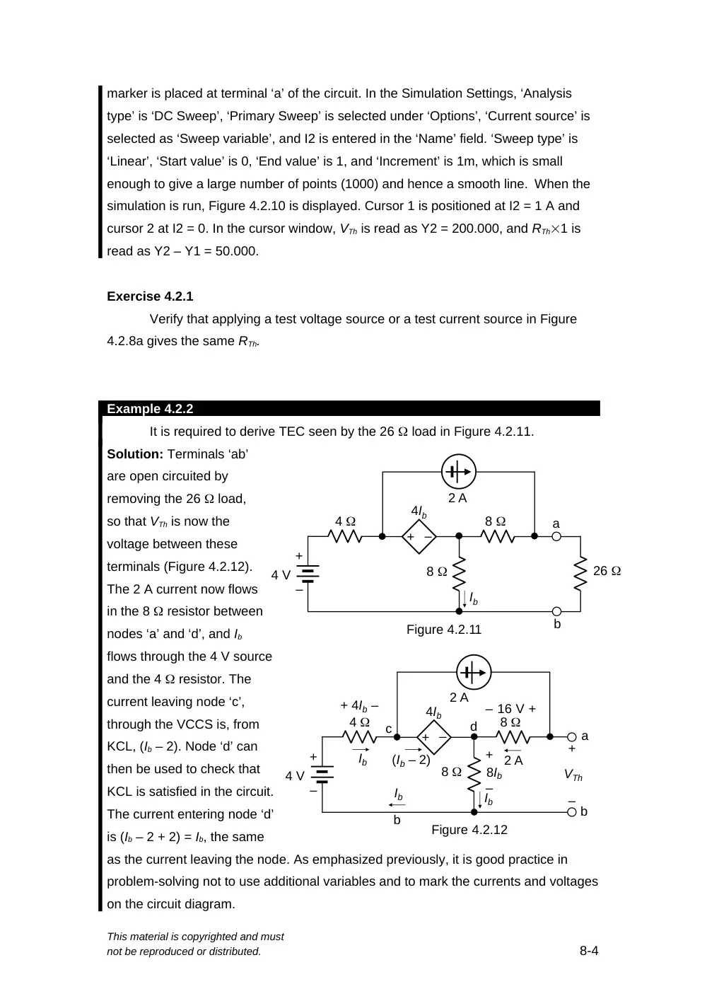7-4 0A 0.5A 1.0A 200V 220V 240V 250V Test current VT Figure 4.2.10 20  30  a b Figure 4.2.8 (a) 50  a b (b) 200 V – + Rin 50  IL 6Adc I2 0Adc 20Vdc 30 20 0 Figure 4.2.9 + _ + - V + - a b marker is placed at terminal ‘a’ of the circuit. In the Simulation Settings, ‘Analysis type’ is ‘DC Sweep’, ‘Primary Sweep’ is selected under ‘Options’, ‘Current source’ is selected as ‘Sweep variable’, and I2 is entered in the ‘Name’ field. ‘Sweep type’ is ‘Linear’, ‘Start value’ is 0, ‘End value’ is 1, and ‘Increment’ is 1m, which is small enough to give a large number of points (1000) and hence a smooth line. When the simulation is run, Figure 4.2.10 is displayed. Cursor 1 is positioned at I2 = 1 A and cursor 2 at I2 = 0. In the cursor window, VTh is read as Y2 = 200.000, and RTh1 is read as Y2 – Y1 = 50.000. Exercise 4.2.1 Verify that applying a test voltage source or a test current source in Figure 4.2.8a gives the same RTh. Example 4.2.2 It is required to derive TEC seen by the 26  load in Figure 4.2.11. Solution: Terminals ‘ab’ are open circuited by removing the 26  load, so that VTh is now the voltage between these terminals (Figure 4.2.12). The 2 A current now flows in the 8  resistor between nodes ‘a’ and ‘d’, and Ib flows through the 4 V source and the 4  resistor. The current leaving node ‘c’, through the VCCS is, from KCL, (Ib – 2). Node ‘d’ can then be used to check that KCL is satisfied in the circuit. The current entering node ‘d’ is (Ib – 2 + 2) = Ib, the same as the current leaving the node. As emphasized previously, it is good practice in problem-solving not to use additional variables and to mark the currents and voltages on the circuit diagram. This material is copyrighted and must not be reproduced or distributed. 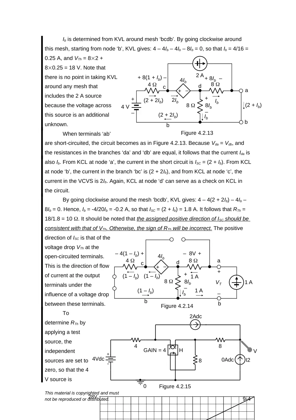8-4 + – 8  8  2 A 4 V 4  – + Ib 4Ib a b + – VTh 2 A Ib Ib (Ib – 2) c d Figure 4.2.12 b + 4Ib – 16 V + + – 8Ib – + – 8  8  26  2 A 4 V 4  – + Ib 4Ib Figure 4.2.11 a b Ib is determined from KVL around mesh ‘bcdb’. By going clockwise around this mesh, starting from node ‘b’, KVL gives: 4 – 4Ib – 4Ib – 8Ib = 0, so that Ib = 4/16 = 0.25 A, and VTh = 82 + 80.25 = 18 V. Note that there is no point in taking KVL around any mesh that includes the 2 A source because the voltage across this source is an additional unknown. When terminals ‘ab’ are short-circuited, the circuit becomes as in Figure 4.2.13. Because Vda = Vdb, and the resistances in the branches ‘da’ and ‘db’ are equal, it follows that the current Ida is also Ib. From KCL at node ‘a’, the current in the short circuit is ISC = (2 + Ib). From KCL at node ‘b’, the current in the branch ‘bc’ is (2 + 2Ib), and from KCL at node ‘c’, the current in the VCVS is 2Ib. Again, KCL at node ‘d’ can serve as a check on KCL in the circuit. By going clockwise around the mesh ‘bcdb’, KVL gives: 4 – 4(2 + 2Ib) – 4Ib – 8Ib = 0. Hence, Ib = -4/20Ib = -0.2 A, so that ISC = (2 + Ib) = 1.8 A. It follows that RTh = 18/1.8 = 10 . It should be noted that the assigned positive direction of ISC should be consistent with that of VTh. Otherwise, the sign of RTh will be incorrect. The positive direction of ISC is that of the voltage drop VTh at the open-circuited terminals. This is the direction of flow of current at the output terminals under the influence of a voltage drop between these terminals. To determine RTh by applying a test source, the independent sources are set to zero, so that the 4 V source is This material is copyrighted and must not be reproduced or distributed. 9-4 + – 8  8  2 A 4 V 4  – + Ib 4Ib a b 2Ib c d Figure 4.2.13 b Ib (2 + Ib) (2 + 2Ib) (2 + 2Ib) + 8(1 + Ib) – + 8Ib – + – 8Ib 8  8  4  – + Ib 4Ib a b + – VT 1 A (1 – Ib) c d Figure 4.2.14 b 1 A 1 A (1 – Ib) (1 – Ib) – 4(1 – Ib) + – 8V + + – 8Ib 4Vdc 4 8 8 0 GAIN = 4 2Adc I2 0Adc V H + - + - Figure 4.2.15 + - + - 28V Figure 4.2.17 + – 5 V 25  10  30  15  20  b c d (a) + – 5 V 30  20  a b c d (b) + – + – 3 V 3 V 10  15  replaced by a short circuit and the 2 A source by an open circuit, as shown in Figure 4.2.14. With a 1 A test source applied, KCL is satisfied at node ‘d’ by having a current (1 – Ib) leaving this node through the VCVS and the 4  resistor. Node ‘b’ can be used to check KCL. By going clockwise around the mesh ‘bcdb’, KVL gives: 4(1 – Ib) – 4Ib – 8Ib = 0. Hence, Ib = 4/16 = 0.25 A, and VT = 81 + 80.25 = 10 V. It follows that RTh = (10 V)/(1 A) = 10 , as before. Simulation: The circuit is entered as in Figure 4.2.15. Proceeding as in Example 4.2.1, Figure 4.2.16 is displayed when the simulation is run. It is seen that VTh = 18 V and RTh = 10 . Problem-Solving Tip  In deriving TEC, the assigned positive direction of ISC should be in the direction of the voltage drop VTh so as to obtain the correct sign of RTh = VTh/ISC. Exercise 4.2.2 Determine RTh in Figure 4.2.14 by applying a 1 V test source rather than a 1 A source. Example 4.2.3 It is required to derive TEC seen by the 25  resistor in Figure 4.2.17a. Solution: As mentioned previously, the circuit configuration is a bridge circuit, since the 25  resistor between nodes ‘c’ and ‘d’ is a “crossover” element, like a bridge. To derive TEC seen by the 25  resistor, the resistor is removed and Vbc determined (Figure 4.2.17b). The voltages Vbd and Vcd in Figure 4.2.17b can be determined from voltage division, since the 10  resistor is in series with the 15  resistor, and the 20  resistor is in series with the 30  resistor. Hence, Vbd = 530/(20 + 30) = 3 V, and Vcd = 515/(10 + 15) = 3 V. When the two middle nodes of the bridge circuit are at the same voltage, that This material is copyrighted and must not be reproduced or distributed. 10-4 is, Vbd = Vcd, the bridge is said to be “balanced”, as will be discussed more fully in Appendix 5A, Chapter 5. With the bridge balanced, VTh = Vbc = Vbd – Vcd = 0. Moreover, when nodes ‘b’ and ‘c’ are at the same voltage, then the current through any resistor connected between these nodes is zero, because there is no voltage to drive such a current. The current remains zero as the resistance is reduced to zero, that is, when nodes ‘b’ and ‘c’ are short circuited. It follows that ISC = 0. However, having VTh and ISC equal to zero does not mean that RTh = 0, because RTh = VTh/ISC is indeterminate and could be finite. To determine RTh, therefore, the resistance looking into terminals ‘bc’ should be derived, with the independent voltage source set to zero, that is, replaced by a short- circuit (Figure 4.2.18a). To make it easier to visualize the connections, it is helpful to redraw the circuit as in Figure 4.2.18b. Clearly, the resistance between nodes ‘c’ and ‘d’ is (10||15 + 20||30) = 18 . With VTh = 0, TEC reduces to an 18  resistor. Simulation: The circuit is entered as in Figure 4.2.19. Proceeding as in Example This material is copyrighted and must not be reproduced or distributed. 11-4 0A 0.2A 0.4A 0.6A 0.8A 1.0A 0V 5V 10V 15V 20V Test current VT Figure 4.2.20 30  20  a b c d (a) 10  15  Figure 4.2.18 c a, d 10  15  30  20  b (b) 5Vdc 20 10 30 15 0Adc 0 V + - Figure 4.2.19 + - 4.2.1, Figure 4.2.20 is displayed when the simulation is run. It is seen that VTh = 0 and RTh = 18 . Example 4.2.4 It is required to determine IX in Figure 4.2.21 using TEC. Solution: TEC will be derived in two steps. The first step is to determine TEC as seen by the 3 A source in parallel with the 6  resistor, as illustrated in Figure 4.2.22a. The motivation for this step is that the parallel combination of the 3 A source and the 6  resistor is connected between the terminals where TEC is required. Under these conditions this parallel combination can be temporarily removed, resulting in a considerably simpler circuit for which an intermediate TEC can be more easily derived. The 3 A source is then be added to this intermediate TEC and a new TEC derived, from which IX is determined by adding the 6  resistor. It is seen from voltage division in Figure 4.2.22a that Vac = 96/9 = 6 V, and Vbc = 93/9 = 3 V. It follows that VTh1 = Vac – Vbc = 6 – 3 = 3 V. RTh1 is most easily found by determining the resistance between terminals ‘ab’ with the 9 V source set to zero, that is, replaced by a short circuit. This makes RTh1 = Rab = (6||3) + (6||3) = 2 + 2 = 4 . The intermediate TEC will therefore consist of VTh1 = 3 V is series with RTh1 = 4  (Figure 4.2.22b). The next step is to connect the 3 A current source and derive a second TEC as seen by the 6  resistor (Figure 4.2.23a). The 3A current now flows through the 3 V source and the 4  resistor, so that the open-circuit voltage Vab = VTh2 = 3 + 12 = This material is copyrighted and must not be reproduced or distributed. 12-4 Figure 4.2.22 9 V 6  6  3  3  a b c + – 6 V + – 3 V (a) 4  (b) + – + – 3 V a b Figure 4.2.21 9 V 6  6  3  3  6  3 A IX + – 15 V. When the 3 A source is replaced by an open circuit and the 3 V source by a short circuit, the resistance seen between terminals ‘ab’ is RTh2 = Rab = 4  as before (Figure 4.2.23b). When the 6  resistor is connected to terminals ‘ab’, IX that flows is 15/(6 + 4) = 1.5 A (Figure 4.2.23c). Simulation: Although the current IX can be derived directly by simulating the circuit of Figure 4.2.21 without invoking TEC, it is instructive to derive by simulation TEC as seen by the 6  resistor. The circuit is entered as in Figure 4.2.24. Proceeding as in Example 4.2.1, Figure 4.2.21 is displayed when the simulation is run. It is seen that VTh = 15 V and RTh = 4 , as determined previously. Problem- Solving Tips  When a voltage or a current in a circuit is required, it can often be conveniently determined by deriving TEC at the terminals associated with this voltage or current.  In deriving TEC it is often advantageous to temporarily remove elements that appear in parallel or in series with the terminals between which TEC is required, derive an intermediate TEC, then restore the removed elements to this intermediate TEC in order to derive the final TEC. This material is copyrighted and must not be reproduced or distributed. 13-4 0A 0.2A 0.4A 0.6A 0.8A 1.0A 15V 16V 17V 18V 19V Test current VT Figure 4.2.25 Figure 4.2.24 9Vdc 6 3 0 3 6 3Adc 0Adc V + - + - + - Figure 4.2.23 (a) 4  (b) + – 3 V a b 4  + – 15 V a b 3 A 3 A + – 12 V (c) 4  + – 15 V a b 6  IX Exercise 4.2.3 Determine RTh in Figure 4.2.22a by deriving ISC. Primal Exercise 4.2.4 Determine TEC between nodes ‘a’ and ‘b’ in Figure 4.2.26: (a) without including the 60  resistance between these nodes; (b) including this resistance. Ans. (a) 12 V in series with 30 ; (b) 8 V in series with 20 . 4.3 Norton’s Theorem In the context of resistive circuits, Norton’s theorem can be stated as follows: Statement: A circuit consisting of ideal resistors and sources is equivalent, at a specified pair of terminals, to a linear-output current source. It is seen that Norton’s equivalent circuit (NEC) is in fact the linear- output current source equivalent of TEC. The two equivalent circuits are related by source transformation, as illustrated in Figure 4.3.1. The ideal current source IN is referred to as Norton’s current and is the short-circuit current of TEC, that is, VTh/RTh, in accordance with source transformation. The source resistance that is in parallel with IN is Norton’s resistance RN, and is the same as RTh in TEC. It is sometimes more convenient to derive NEC rather than TEC, as in Example 4.3.1. Moreover, some circuits may have an NEC but not a TEC, or conversely, as in the case of ideal voltage sources and ideal current sources. Thus, an ideal voltage source can be considered to be its own TEC, with RTh = 0. IN = VTh/0  , which means that NEC does not exist. Similarly, an ideal current source can be regarded as its own NEC, with RN = , so that VTh  , which means that TEC does not exist. This is in accordance with the fact that an ideal voltage source cannot be This material is copyrighted and must not be reproduced or distributed. 14-4 a RL + – VTh RTh b (a) (b) a b RL IN RN RTh = RN VTh = RNIN Figure 4.3.1 Figure 4.2.26 + – 20 V 6  60  60  40  a b transformed to an ideal current source, and conversely, as explained in Section 3.6, Chapter 3. Circuits that have TEC but not NEC generally reduce to an ideal voltage source between the terminals involved, whereas circuits that have NEC but not TEC generally reduce to an ideal current source between these terminals. Examples of these are given in the problems at the end of the chapter. The procedure for deriving NEC is essentially the same as that for TEC. When independent sources are set to zero in Figure 4.3.1, the ideal voltage source in TEC is replaced by a short circuit and the ideal current source in NEC is replaced by an open circuit. The resistance looking into terminals ‘ab’ is RTh = RN in both cases. In the case of TEC, VTh is generally determined directly, and the short-circuit current, IN, is determined as an alternative method for finding RTh. In the case of NEC, IN is generally determined directly, and the open-circuit voltage, VTh, is determined as an alternative method for finding RN. Derivation of NEC with PSpice NEC can be derived in a single simulation, analogous to that described for TEC, and explained in Figure 4.3.2a. A test source VT is connected between these terminals with the circuit left as is, that is with the independent sources retained, so that IN  0. KCL gives: (4.3.1) If VT is varied between 0 and 1 V, and IT is plotted against VT, a straight line graph is obtained having a current intercept IN at VT = 0. The difference between IT1, which is IT at VT = 1 V, and IN is numerically equal to GN (Figure 4.3.2b). VT is conveniently varied in PSpice over a desired range of values, using the “DC Sweep” feature. Example 4.3.1 It is required to determine IL in Figure 4.3.3 using NEC. This material is copyrighted and must not be reproduced or distributed. 15-4 (a) + – VT (b) VT IN Slope = GN 1 A 0 IT1 = IN + GN1 IT Figure 4.3.2 GN IN GN GNVT IT IT1 – – + + 15  10  5 A 2VX VX IS 3IS 50  IL Figure 4 3 3 a b Solution: When terminals ‘ab’ are short circuited, VX = 0 and the VCVS becomes a short circuit (Figure 4.3.4a). The 15  and 10  resistors are paralleled. By current division, the currents in these two resistors are 2 A and 3 A as shown. IS = -2 A and the CCCS becomes 6 A directed upwards. It follows that ISC = IN = 3 + 6 = 9 A. Note that the 6 A source current only adds to the current in the short circuit between nodes ‘a’ and ‘b’ in Figure 4.3.4a and does not affect current division. To determine RN, a test source IT is applied, with the 5 A current source replaced by an open circuit (Figure 4.3.4b). KVL gives: 2VT – 25IS –VT = 0, or VT = 25IS (4.3.2) From KCL, IS + IT = 3IS, or, IT = 2IS (4.3.3) Dividing Equation 4.3.3 by Equation 4.3.2,  (4.3.4) NEC therefore consists of a 9 A source in parallel with a 12.5  resistor (Figure 4.3.5a). When the 50  resistor is connected between terminals ‘ab’, it follows from current division that: = 1.8 A (4.3.5) It may be noted that determining the open-circuit voltage in Figure 4.3.3 in order to work with TEC is slig