EECE 340 Exam 1, Spring 2016

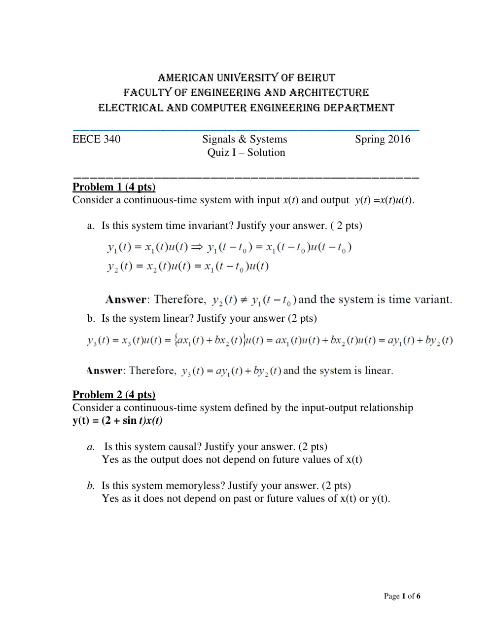
Page 1 of 6 AMERICAN UNIVERSITY OF BEIRUT FACULTY OF ENGINEERING AND ARCHITECTURE ELECTRICAL AND COMPUTER ENGINEERING DEPARTMENT ___________________________________________ EECE 340 Signals & Systems Spring 2016 Quiz I – Solution ___________________________________________ Problem 1 (4 pts) Consider a continuous-time system with input x(t) and output y(t) =x(t)u(t). a. Is this system time invariant? Justify your answer. ( 2 pts) b. Is the system linear? Justify your answer (2 pts) Problem 2 (4 pts) Consider a continuous-time system defined by the input-output relationship y(t) = (2 + sin t)x(t) a. Is this system causal? Justify your answer. (2 pts) Yes as the output does not depend on future values of x(t) b. Is this system memoryless? Justify your answer. (2 pts) Yes as it does not depend on past or future values of x(t) or y(t). Page 2 of 6 Problem 3 (4 pts) f(t) Write the time domain representation of the derivative of the above signal f(t). )1 6 ( 3 2 6 3 2 2 3 1 2 3 1 6 6 ( ) ( )                            u t u t t t t u t dt df t   Grading policy: -1 -1 -1 -1 Problem 4 (4 pts) Consider the system represented by the following block diagram Is it possible to represent this system with a linear differential equation with constant coefficients? If yes, derive this differential equation. Answer As every integrator has a transfer function of 1/s, the transfer function of the system using Mason’s rule is: s s s s s s X s Y 4 1 3 1 1 1 ) ( ) ( 3 2 2 3             , That is ( ) ( ) 4 3 ( ) X s sY s s Y s   Using Laplace Transform with zero Initial conditions ( ) ( ) 4 ( ) 3 3 x t dt t dy dt d y t   Grading Policy: Matrix representation -3 Page 3 of 6 Problem 5 (4 pts) Consider a continuous-time LTI system which has impulse response of )1 ( ( ) ( )    u t u t h t . If 3)] ( [ ( ) ( )    u t t u t x t is applied at the input of the system, evaluate the output y(t). Answer s e s H s u t u t t h s        1 ( ) )1 ( ( ) ( ) 1 pt s e s e s X s u t u t t tu t t x s s 3 2 3 2 3 1 ( ) 3) 3 ( 3) 3) ( ( ( ) ) (             1 pt 2 4 2 23 3 4 3 3 3 3 3 3 1 ( ) ( ) ) ( s e s e s e s e s e s X s H s s Y s s s s                                    4) 4) ( 6( 3) 3) ( ( 6 4) ( 4) ( 3) ( 3) ( )1 ( )1 ( ) ( 2 1 ) ( 2 2 2 2 u t t u t t u t t u t t u t t t u t y t 2 pts Problem 6 (5 pts) For the system shown above, determine a differential equation that relates the input x(t) and output y(t) of the closed loop system. Solution The forward transfer function 6 5 1 ( ) 2     s s s G s The closed-loop Transfer function 8 7 1 ) ( ) ( 2     s s s s X Y s The corresponding Differential equation ( ) ( ) 8 ( ) ( ) 7 ( ) 3 2 x t dt dx t y t dt t dy dt d y t     Incorrect coefficient -1 Page 4 of 6 Problem 7 (5 pts) Two linear time-invariant systems connected in series as shown below The differential equations given below represent the input-output relationships for each system ( ) ( ) ( ) d 2 2 x t t y dt y t   and dt dy t z t dt z t ( ) 6 ( ) d ( )   Find the transfer function of the system. Solution System 1: 1 1 ) ( Y(s) ( ) 2 1    s X s G s 1 pt System 2: 6 ) ( Z(s) 2 ( )    s s Y s s G 1 pt Overall System Transfer function:   6 1 ) ( Z(s) ( ) 2     s s s X s G s 2 pts Problem 8 (5 pts) The forward transfer of a unity feedback control system is given by 6) 2)(s (s (s-7) G(s) 2     s Use the Routh-Hurwitz stability criterion to determine the location of the poles of the system in each half of the complex plane. 5 5 7 7) ( 6) 2)(s (s (s-7) Input Output 2 3 2            s s s s s s 2 pts 3 s 1 5 2 s 1 5 1s 0 1s 2 3 s 5 s s 2 ds dA(s) 5 A(s) 2     . 5 0 A(s) j s     Table and A(s): 2pts Pole locations (1, 2, 0) 1 pt If RH table is done for the open-loop system, -4 pts Page 5 of 6 Problem 9 (5 pts) Consider the system below and let p=0. Determine conditions on K and z so that the system is stable. Answer Closed-loop TF: Kz Ks s s F       2 3 4 8 2 s z) K(s T 2 pts RH Table (2 pts) 4 s 1 8 Kz 3 s 2 K 2 s 2 16  K Kz 1s K K z K    16 ) 4 (16 0 s Kz 1. 0<K<16 2. 0<z<4 2 pts Problem 10 (5 pts) Determine the Transfer function of the LTI system whose block diagram is shown below. 3 2 1 2 1 1 1 2 1 1 1 3 1 2 1 ) 1( ) ( ) ( G G H G H H G G H G H G G G s R s Y        -1 for every missing or wrong term 1 s(s2+2s+8) + - K(s+z) s+p 1 s(s2+2s+8) + - K(s+z) s+p Page 6 of 6 Problem 11 (5 pts) An LTI system is represented by the following differential equation relating the input r(t) to the output y(t). 5 ( ) ( ) 3 ( ) 4 6 ( ) ( ) 5 ( ) 3 ( ) 8 2 2 2 2 3 3 r t dt t dr dt d r t y t dt t dy dt y t d dt d y t       Represent the system in a state space format Answer ) ( /8 5 /8 3 /8 4 ) ( ) ( ) ( 0 0 /8 6 1 0 /8 5 0 1 /8 3 ) ( ) ( ) ( 3 2 1 3 1 2 t r t X t X t X t X t X t X                                                    ( ) 0 ) ( ) ( ) ( 0 0 1 ) ( 3 2 1 t r t X t X t X y t             -1 for every incorrect term or missing term in a matrix