EECE 460 Homework, Spring 2007

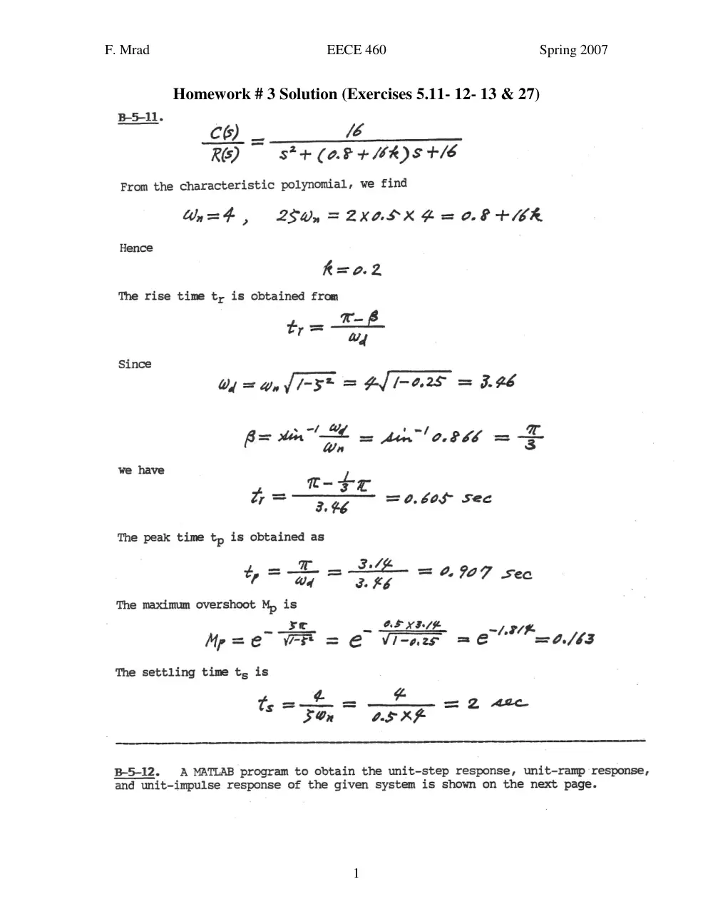
F. Mrad EECE 460 Spring 2007 Homework # 3 Solution (Exercises 5.11- 12- 13 & 27) B-5-ll. C6) lé — = RS) S*+ (0.8 +/HR)STE From the characteristic polynomial, we find Ln=F4 , 25, = 2X0SX4= 0.8 +16R Hence R=0.2 The rise time ty is obtained from ty, = a = Since Oy = yf /-5* = AL -0.2F = 3.96 _ . 1 & _ tw/ _ a A= tm ae = 4in 0.866 =m 3 we have t-$x Z = Fae Obed See The peak time tp is obtained as 4 %=— a ee = 0.907 seo Wd ~ 3.k6 The maximum overshoot Mp is - 5 - OF X3SE -/,8/% Mp=e wr = € Vi-azr RE =30./63 The settling time t, is ts = 4 = —_* = 2 acc Sn 0.5 *F B-5-12. A MATLAB program to obtain the unit-step response, unit-ramp response, and unit-impulse response of the given system is shown on the next page. F. 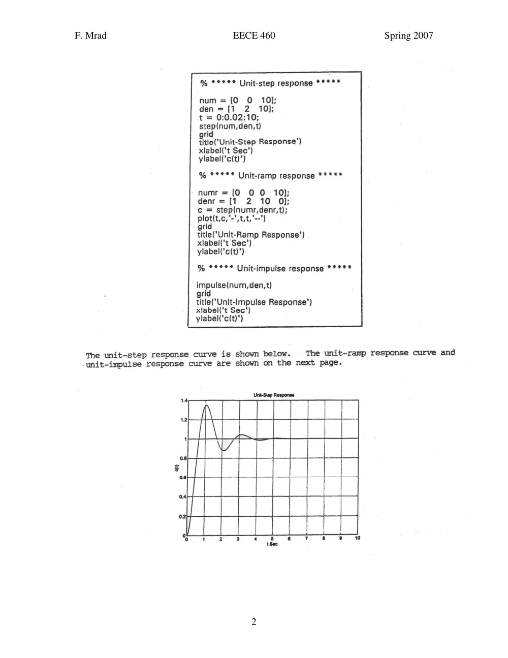Mrad EECE 460 Spring 2007 % ***** Unit-step response ***** num = [0 O 10]; den =[1 2 10]; t = 0:0.02:10; step(num,den,t) grid title("Unit-Step Response’) xlabel('t Sec") ylabel('c(t)’) % ***** Unit-ramp response ***** numr = [0 0 0 10); denr=[1 2 10 0}; c = step(numr,denr,t); plot(t,c,'-',t,t,"--" grid title("'Unit-Ramp Response’) xlabel('t Sec’) ylabel(*c(t)') % ***** Unit-impulse response ***** impulse(num,den,t) grid title("Unit-Impulse Response’) xlabel("t Sec’) ylabel('c(t)') The unit-step response curve is shown below. The unit-ramp response curve and -unit-impulse response curve are shown on the next page. 1.4) A “TT TO. 4 12, 1 \ oe et) F. Mrad EECE 460 Spring 2007 Unit-Ramp Response Unit-impuise Response 25; T 1 2A 15 1 ; - — 1 s | | os) t) PT ; - — ! os Vv _ wot | | L o 1. 2 oo 4 5S 6 7 686 98 10 B-5-13. A MATLAB program to obtain a unit-step response of the given system is given below. The resulting unit-step response curve is shown on the next page. % ***** Unit-Step Response ***** A={[-1 -0.5;1 0]; B = [0.5;0]; C=[1 0}; D = [0]; [y,x,t] = step(A,B,C,D); ploti(t,y) grid title("Unit-Step Response’) xlabel('t Sec’) ylabel(‘Output') F. 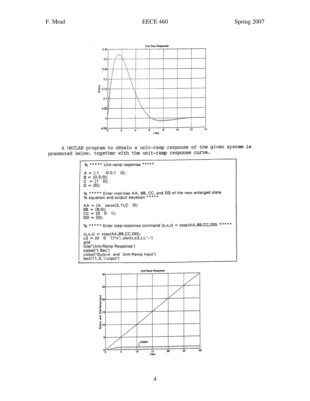Mrad EECE 460 Spring 2007 Unit-Step Response 0.35 T 0.3} oe 0.25}---—- \ 0.2 3 | all \L ~ °° H | | 0.1 a 0.05) tSec A MATLAB program to obtain a unit-ramp response of the given system is presented below, together with the unit-ramp response curve. % ***** Unit-ramp response ***** A=[-1 -0.5;1 0]; B = [0.5;0]; Cc =({1 O}; D = (0); % ***** Enter matrices AA, BB, CC, and DD of the new enlarged state % equation and output equation ***** AA = [A_zeros(2,1);C 0]; BB = [B;0]; cc ={[0 0 1]; DD = [0]; eenee % ***** Enter step-response command [z,x,t] = step(AA,BB,CC,DD) [z,x,t] = step(AA,BB,CC,DD); x3 = {0 O 1]*x'; plot(t,x3,t,t,'--') grid title('Unit-Ramp Response’) xlabei('t Sec’) ylabel('Output and Unit-Ramp Input’) text(11,3,'Uutput’) {aoe _ Uni-Ramp Response 25| En E & 31 3 gr 5 + Output 0 + 0 5 10 15 20 25 Ko) tSec F. 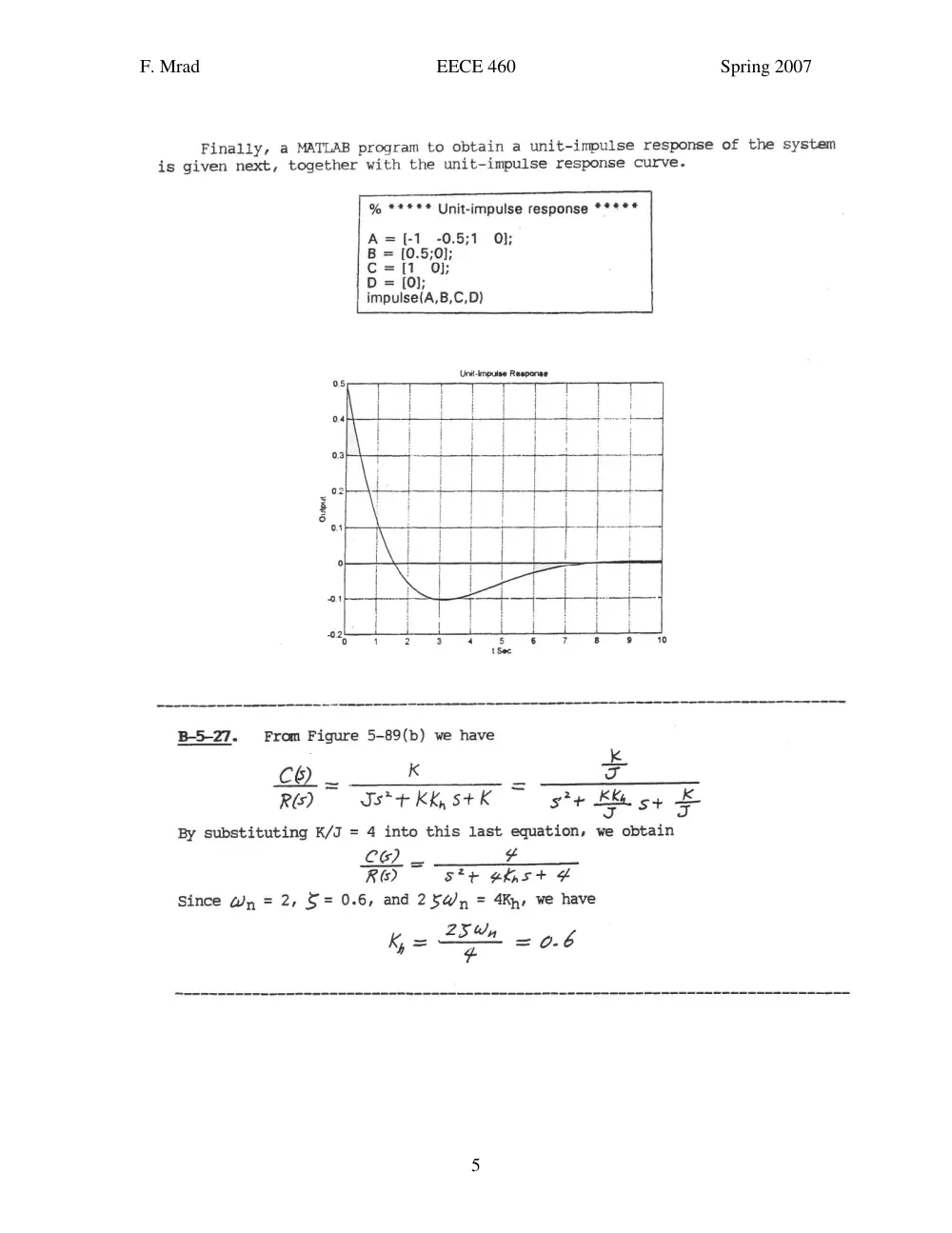Mrad EECE 460 Spring 2007 Finally, a MATLAB program to obtain a unit-impulse response of the system is given next, together with the unit-impulse response curve. % ***** Unit-impulse response ***** -1 -0.5;1 0]; I B-5-27. From Figure 5-89(b) we have a CH _. K _ Z RG) Js*+ Kk, 5+K srt co st £ By substituting K/J = 4 into this last equation, we obtain CO) _ $ R@® Str aehyst Since Wy = 2, $= 0.6, and 2 5@y, = 4Kp, we have 25 Wy Z K, = = 0.6