EECE 460 Homework, Spring 2008

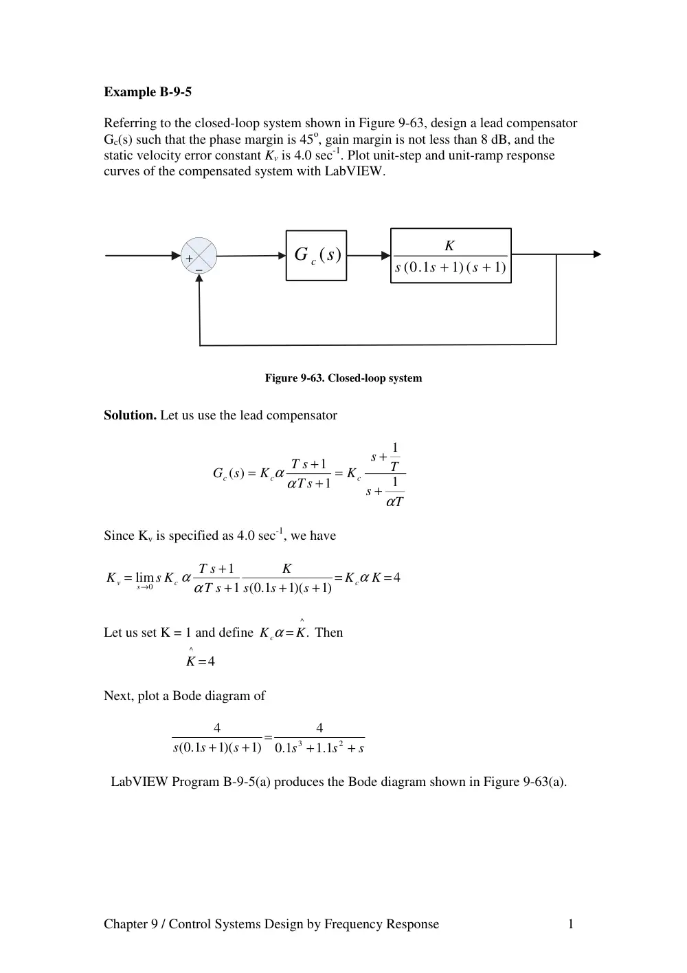
Chapter 9 / Control Systems Design by Frequency Response 1 Example B-9-5 Referring to the closed-loop system shown in Figure 9-63, design a lead compensator Gc(s) such that the phase margin is 45o, gain margin is not less than 8 dB, and the static velocity error constant Kv is 4.0 sec-1. Plot unit-step and unit-ramp response curves of the compensated system with LabVIEW. + − 1) 1) ( (0 1. + + s s s K (s) G c Figure 9-63. Closed-loop system Solution. Let us use the lead compensator T s T s K T s T s K s G c c c α α α 1 1 1 1 ( ) + + = + + = Since Kv is specified as 4.0 sec-1, we have 4 )1 1)( 1 ( 1.0 1 lim 0 = = + + + + = → K K s s s K T s T s s K K c c s v α α α Let us set K = 1 and define ^ K. 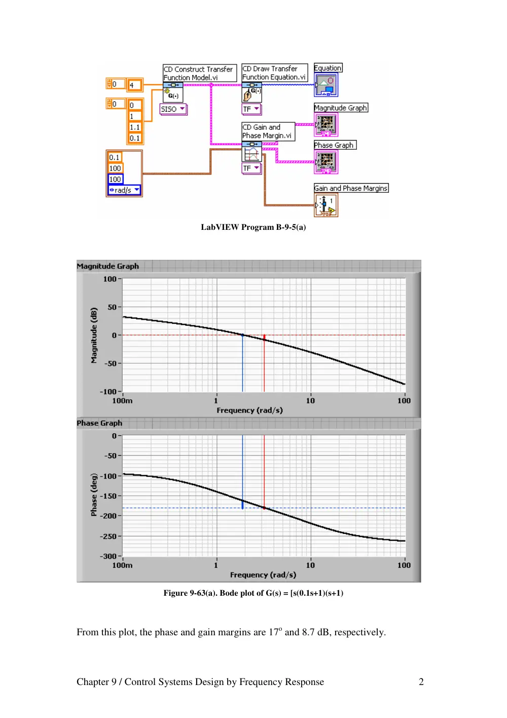K c α = Then 4 ^ K = Next, plot a Bode diagram of s s s s s s + + = + + 2 3 1.1 1.0 4 )1 1)( ( 1.0 4 LabVIEW Program B-9-5(a) produces the Bode diagram shown in Figure 9-63(a). Chapter 9 / Control Systems Design by Frequency Response 2 LabVIEW Program B-9-5(a) Figure 9-63(a). Bode plot of G(s) = [s(0.1s+1)(s+1) From this plot, the phase and gain margins are 17o and 8.7 dB, respectively. Chapter 9 / Control Systems Design by Frequency Response 3 Since the specifications call for a phase margin of 45o, let we choose ο ο ο ο φ 40 12 17 45 = + − m = (This means that 12o has been added to compensate for the shift in the gain crossover frequency.) The maximum phase lead is 40o. Since 40 ) ( 1 1 sin ο ϕ α α ϕ = + − = m m α is determined as 0.2174. Let us choose, instead of 0.2174, α to be 0.21, or α = 0.21 Next step is to determine the corner frequencies ω=1/T and ω=1/ (αT) of the lead compensator. Note that the maximum phase-lead angle φm occurs at the geometric mean of the two corner frequencies, or ) 1/( αT ω = . The amount of the modification in the magnitude curve at ) 1/( αT ω = due to the inclusion of the term (T s+1)/( αTs+1) is α ωα ω α ω 1 1 1 ) 1/( = + + = T T j j T Note that . .6 7778 21 .0 1 1 dB = = α We need to find the frequency point where, when the lead compensator is added, the total magnitude becomes 0 dB. The magnitude of G(jω) is -6.7778 dB corresponds to ω = 2.81 rad/sec. We select this frequency to be the new gain crossover frequency ωc. Then we obtain .1 2877 .2 81 .0 21 1 = = = x T α ωc .6 1319 21 .0 .2 81 1 = = = α ω α c T Hence .6 1319 .1 2877 ( ) + + = s K s s G c c and .0 21 4 ^ = α = K K c Chapter 9 / Control Systems Design by Frequency Response 4 Thus 1 16308 .0 1 .0 7766 4 .6 1319 2877 .1 .0 21 4 ( ) + + = + + = s s s s Gc s The open-loop transfer function becomes as s s s s s s s s s s s G s Gc + + + + = + + + + = 2 3 4 .1 2631 .0 2794 .0 01631 4 1064 .3 )1 1)( ( 1.0 1 1 .0 16308 1 .0 7766 4 ( ) ) ( the closed-loop transfer function is 4 .4 1064 .1 2631 .0 2794 .0 01631 4 .3 1064 ( ) ) ( 2 3 4 + + + + + = s s s s s R s C s 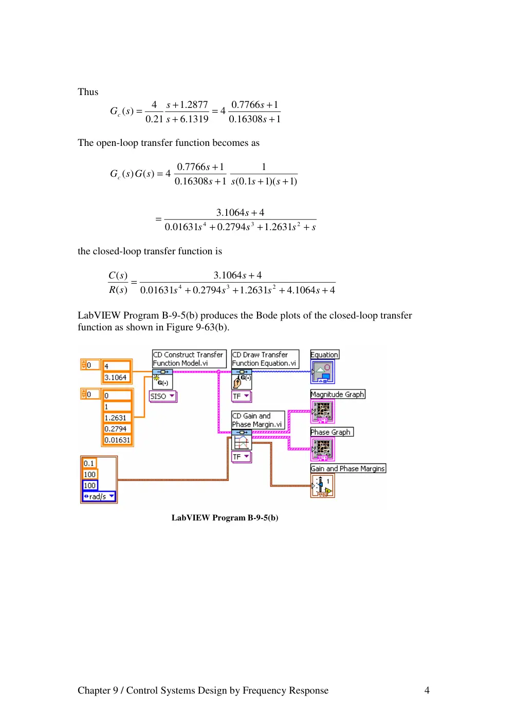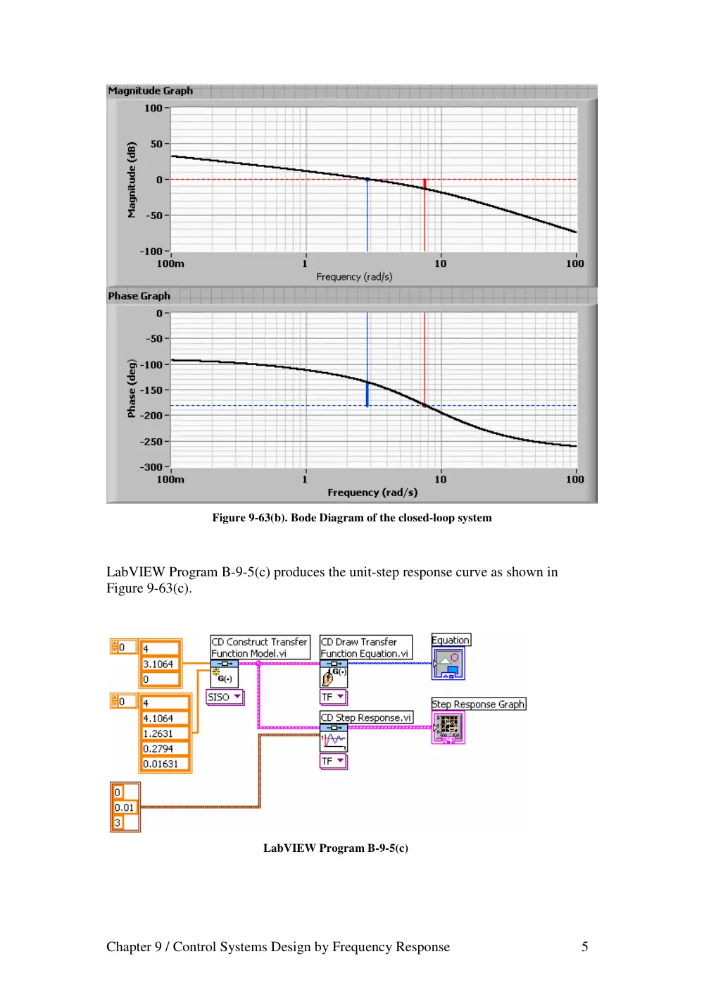LabVIEW Program B-9-5(b) produces the Bode plots of the closed-loop transfer function as shown in Figure 9-63(b). LabVIEW Program B-9-5(b) Chapter 9 / Control Systems Design by Frequency Response 5 Figure 9-63(b). 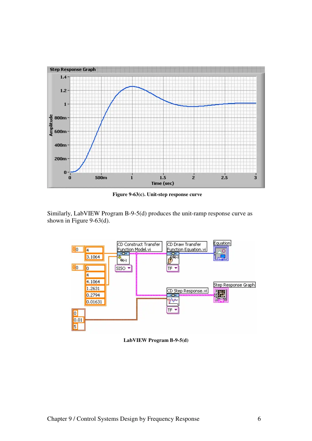Bode Diagram of the closed-loop system LabVIEW Program B-9-5(c) produces the unit-step response curve as shown in Figure 9-63(c). LabVIEW Program B-9-5(c) Chapter 9 / Control Systems Design by Frequency Response 6 Figure 9-63(c). 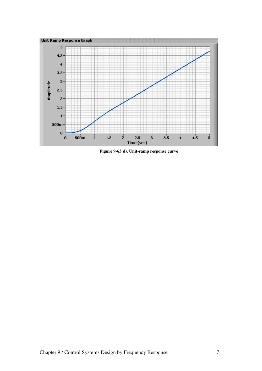Unit-step response curve Similarly, LabVIEW Program B-9-5(d) produces the unit-ramp response curve as shown in Figure 9-63(d). LabVIEW Program B-9-5(d) Chapter 9 / Control Systems Design by Frequency Response 7 Figure 9-63(d). 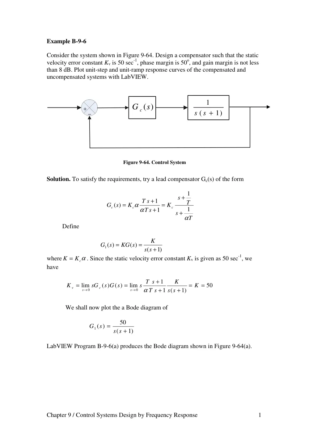Unit-ramp response curve Chapter 9 / Control Systems Design by Frequency Response 1 Example B-9-6 Consider the system shown in Figure 9-64. Design a compensator such that the static velocity error constant Kv is 50 sec-1, phase margin is 50o, and gain margin is not less than 8 dB. Plot unit-step and unit-ramp response curves of the compensated and uncompensated systems with LabVIEW. + − 1) ( 1 s s + (s) G c Figure 9-64. Control System Solution. To satisfy the requirements, try a lead compensator Gc(s) of the form T s T s K T s T s K s G c c c α α α 1 1 1 1 ( ) + + = + + = Define )1 ( ( ) 1 ( ) + = = s s K KG s G s where K = Kcα . 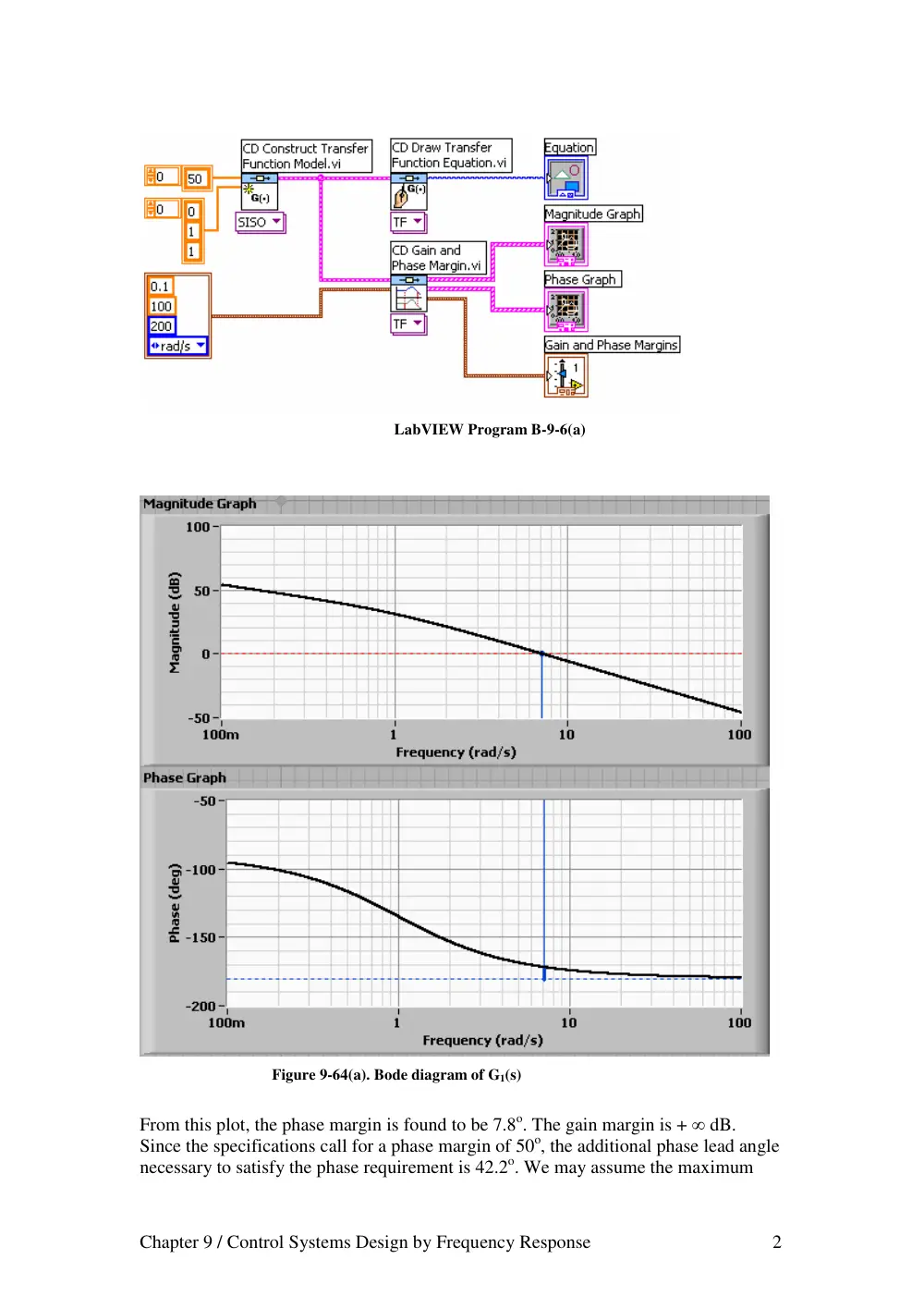Since the static velocity error constant Kv is given as 50 sec-1, we have 50 1) 1 ( 1 lim ( ) ( ) lim 0 0 = = + + + = = → → K s s K T s s T s s G s sG K s c s v α We shall now plot the a Bode diagram of 1) ( 50 ) 1 ( + = s s s G LabVIEW Program B-9-6(a) produces the Bode diagram shown in Figure 9-64(a). Chapter 9 / Control Systems Design by Frequency Response 2 LabVIEW Program B-9-6(a) Figure 9-64(a). Bode diagram of G1(s) From this plot, the phase margin is found to be 7.8o. The gain margin is + ∞ dB. Since the specifications call for a phase margin of 50o, the additional phase lead angle necessary to satisfy the phase requirement is 42.2o. 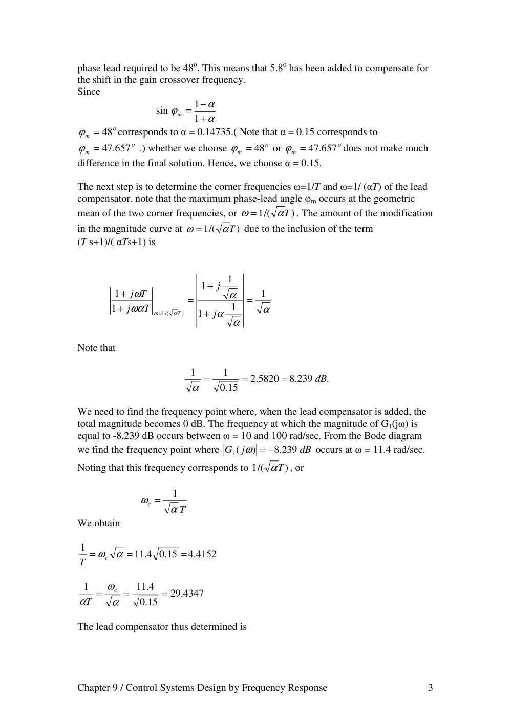We may assume the maximum Chapter 9 / Control Systems Design by Frequency Response 3 phase lead required to be 48o. This means that 5.8o has been added to compensate for the shift in the gain crossover frequency. Since α α ϕ + − = 1 1 sin m ο ϕ m = 48 corresponds to α = 0.14735.( Note that α = 0.15 corresponds to ο ϕ m = 47.657 .) whether we choose ο ϕ m = 48 or ο ϕ m = 47.657 does not make much difference in the final solution. Hence, we choose α = 0.15. The next step is to determine the corner frequencies ω=1/T and ω=1/ (αT) of the lead compensator. note that the maximum phase-lead angle φm occurs at the geometric mean of the two corner frequencies, or ) 1/( αT ω = . The amount of the modification in the magnitude curve at ) 1/( αT ω = due to the inclusion of the term (T s+1)/( αTs+1) is α α α α ωα ω α ω 1 1 1 1 1 1 1 ) 1/( = + + = + + = j j T j T j T Note that . .8 239 .2 5820 15 .0 1 1 dB = = = α We need to find the frequency point where, when the lead compensator is added, the total magnitude becomes 0 dB. The frequency at which the magnitude of G1(jω) is equal to -8.239 dB occurs between ω = 10 and 100 rad/sec. From the Bode diagram we find the frequency point where dB j G .8 239 ) 1( = − ω occurs at ω = 11.4 rad/sec. Noting that this frequency corresponds to ) 1/( αT , or T c α ω 1 = We obtain .4 4152 .0 15 11 4. 1 = = = ωc α T 29.4347 15 .0 11 4. 1 = = = α ω α c T The lead compensator thus determined is Chapter 9 / Control Systems Design by Frequency Response 4 29.4347 .4 4152 1 1 ( ) + + = + + = s s K T s T s K s G c c c α Where Kc is determined as 3 1000 .0 15 = α = 50 = K K c Thus, 1 03397 .0 1 .0 2265 50 .4347 29 4152 .4 3 1000 ( ) + + = + + = s s s s Gc s LabVIEW Program B-9-6(b) produces the Bode diagram of the lead compensator just designed, as shown in Figure 9-64(b). LabVIEW Program B-9-6(b) Chapter 9 / Control Systems Design by Frequency Response 5 Figure 9-64(b). Bode Diagram of Gc(s) The open-loop transfer function of the designed system is )1 ( 1 29.4347 .4 4152 3 1000 ( ) ( ) +       + + = s s s s Gc s G s LabVIEW Program B-9-6(c) produces the Bode diagram of Gc(s)G(s),which is shown in Figure 9-64(c). Chapter 9 / Control Systems Design by Frequency Response 6 LabVIEW Program B-9-6(c) Figure 9-64(c). Bode diagram of Gc(s)G(s), From this diagram, it is clearly seen that the phase margin is approximately 52o, the gain margin is + ∞ dB, and Kv = 50 sec-1 ; all specifications are met. Chapter 9 / Control Systems Design by Frequency Response 7 Next we shall obtain the unit-step and unit-ramp responses of the original uncompensated system and the compensated system. The original uncompensated system has the following closed-loop transfer function: 1 1 ( ) ) ( 2 + + = s s R s C s The closed-loop transfer function of the compensated system is 4415 2. 1088.3041 91.3041 3 4415 2. 1000 .4 4152) 1000( )1 29.4347) ( 3( .4 4152) 1000( ( ) ) ( 2 3 + + + + = + + + + + = s s s s s s s s s R s s C The closed-loop poles of the compensated system are as follows: .8 0804 .7 536 .1772 11 .7 5636 .1772 11 = − − − = + − = s j s j s LabVIEW Program B-9-6(d) produces the unit-step responses of the uncompensated and compensated systems. The resulting response curves are shown in Figure 9-64(d). LabVIEW Program B-9-6(d) Chapter 9 / Control Systems Design by Frequency Response 8 Figure 9-64(d). Unit-step responses of the uncompensated and compensated systems. LabVIEW Program B-9-6(e) produces the unit-ramp responses of the uncompensated system and compensated system. The resulting response curves are shown in Figure 9-64(e). LabVIEW Program B-9-6(e) Chapter 9 / Control Systems Design by Frequency Response 9 Figure 9-64(e). Unit-ramp responses of the Uncompensated and Compensated systems. Chapter 9 / Control Systems Design by Frequency Response 1 Example B-9-7 Consider the system shown in Figure 9-65. Design a compensator such that the static velocity error constant is 4 sec-1, phase margin is 50o, and gain margin is 10 dB or more. Plot unit-step and unit-ramp response curves of the compensated system with LabVIEW. Also, draw a Nyquist plot of the compensated system with LabVIEW. + − 1 .1 0 2 + + s s (s) G c Figure 9-65. Control System Solution. Since the plant does not have an integrator, it is necessary to add an integrator in the compensator. Let us choose the compensator to be ( ) ( ) s s G K s G c c = , ( ) 1 lim ^ 0 = → s G c s Where ) ( ^ G c s is to be determined later. Since the static velocity error constant is specified as 4 sec-1, we have 4 1.0 1 1.0 ( ) lim 1 1.0 ( ) lim 2 ^ 0 2 0 = = + + = + + = → → K s s s s G K s s s s sG K c s c s v Thus, K = 40. Hence ( ) 40 ) ( ^ s s G G s c = Next, we plot a Bode diagram of )1 ( )1.0 40( ) ( 2 + + = s s s G s LabVIEW Program B-9-7(a) produces a Bode diagram of G(s) as shown in Figure 9-65(a). Chapter 9 / Control Systems Design by Frequency Response 2 LabVIEW Program B-9-7(a) Figure 9-65(a). Bode diagram of G(s) We need the phase margin of 50o and gain margin of 10 dB or more. Let us choose ) ( ^ G c s to be 0) ( 1 ) ( ^ > + = a a s G c s Chapter 9 / Control Systems Design by Frequency Response 3 Then Gc(s) will contribute up to 90o phase lead in the high frequency region. By simple trials, we find that a = 0.1526 gives the phase margin of 50o and gain margin of + ∞ dB. LabVIEW Program B-9-7(b) produces the Bode diagram of ^ ( ) ( ) s G s G c which is shown in Figure 9-65(b). From this Bode diagram we see that the static velocity error constant is 4 sec-1, phase margin is 50o, and gain margin is + ∞ dB. Therefore the designed system satisfies all the requirements. LabVIEW Program B-9-7(b) Chapter 9 / Control Systems Design by Frequency Response 4 Figure 9-65(b). Bode diagram of ^ ( ) ( ) s G s G c The designed compensator has the following transfer function s s s s G s G c c )1 40( .0 1526 ( ) 40 ) ( ^ + = = The open-loop transfer function of the designed system is )1 ( 4 40.6104 104 .6 )1 ( )1.0 )1 ( ( .0 1526 40 2 2 2 + + + = + + + = − s s s s s s s s loop transfer function Open We shall next check the unit-step response and the unit-ramp response of the designed system. The closed-loop transfer function is Chapter 9 / Control Systems Design by Frequency Response 5 4 41.6104 .6 104 4 40.6104 .6 104 ( ) ) ( 2 3 2 + + + + + = s s s s s R s C s The closed-loop poles are located at .0 0975 .5 6573 0032 .3 .5 6573 0032 .3 =− − − = + − = s j s j s LabVIEW Program B-9-7(c) will produce the unit-step curve of the designed system. The resulting unit-step response curve is shown in Figure 9-65(c). Notice that the closed-loop pole at s = -0.0975 and the plant zero at s = -0.1 produce the long tail of small amplitude. LabVIEW Program B-9-7(c) Figure 9-65(c). Unit-step curve of the designed system Chapter 9 / Control Systems Design by Frequency Response 6 LabVIEW Program B-9-7(d) produces the unit-ramp response curve of the designed system. The resulting response curve is shown in Figure 9-65(d). LabVIEW Program B-9-7(d) Figure 9-65(d). Unit-ramp curve of the designed system. Nyquist plot: Define the open-loop transfer function as G(s). Then )1 ( 4 40.6104 .6 104 1 1.0 ( ) ( ) 2 2 2 + + + = + + = s s s s s s s G G s c Let us choose a modified Nyquist path in the s-plane as shown in Figure (a) below. The modified path encloses three open-loop poles (s = 0, s = j1, s = -j1). Then the Chapter 9 / Control Systems Design by Frequency Response 7 Nyquist path becomes as shown in Figure (b) below. In the s1 plane, the open-loop transfer function has three poles in the right-half s1 plane. Let us choose .0 01. σo = Since s = o s 1 −σ , we have G(s) = g(s1-0.01) Open-loop transfer function in the s1 plane .0 010001 .1 0003 03 .0 .3 5945064 40.48832 104 .6 .1 0001 .0 02 .0 01)( ( 4 .0 01) 40.6104( .0 0001) .0 02 104( .6 1 2 1 3 1 1 2 1 1 2 1 1 1 1 2 1 − + − + + = + − − + − + + − = s s s s s s s s s s s Chapter 9 / Control Systems Design by Frequency Response 8 LabVIEW Program B-9-7(e) is used to obtain the Nyquist plot shown in Figure 9-65(e). LabVIEW Program B-9-7(e) Figure 9-65(e). Nyquist plot Chapter 9 / Control Systems Design by Frequency Response 1 Example B-9-8 Consider the system shown in Figure 9-66. It is desired to design a compensator such that the static velocity error constant is 4 sec-1, phase margin is 50o, and gain margin is 8 dB or more. Plot the unit-step and unit-ramp response curves of the compensated system with LabVIEW. + − 4 1.0 1.0 2 2 + + + s s s G c (s) s 1 1 R Hydraulic Servo Aircraft Rate gyro C Figure 9-66. Control System Solution: The plant transfer function is 4) 0 1. ( 0 1. 2 ) ( 2 + + + = s s s s G s The plant involves a quadratic term with ς = .0 025 . This term is quite oscillatory. LabVIEW Program B-9-8(a) produces the Bode diagram of G(s) as shown in Figure 9-66(a). LabVIEW Program B-9-8(a) Chapter 9 / Control Systems Design by Frequency Response 2 Figure 9-66(a). Bode diagram of G(s) The closed-loop transfer function of the original uncompensated system is 1.0 6 1.0 1.0 2 ( ) ) ( 2 3 + + + + = s s s s R s C s The closed-loop poles of the uncompensated system are .0 0167 .2 4489 0417 .0 .2 4489 0417 .0 =− − − = + − = s j s j s LabVIEW Program B-9-8(b) is used to obtain the unit-step response of this original, uncompensated system. The resulting unit-step response curve is shown in Figure 9-66(b). Chapter 9 / Control Systems Design by Frequency Response 3 LabVIEW Program B-9-8(b) Figure 9-66(b). Unit-step response of uncompensated system To design a compensator for such a system, it is desirable to cancel the zero of the plant, since it is located very close to the origin. It is some-times useful to include double zero and double pole in the compensator. So, we may choose the compensator to be 1.0 2 10) ( 2) ( ( ) 2 2 + + + + = s a s s s K s G c c . Where we have chosen the double zero at s = -2 and double pole at s = -10. The value of a is to be determined later. Since the static velocity error constant is specified as 4 sec-1, we have Chapter 9 / Control Systems Design by Frequency Response 4 4 100 4) 1.0 ( 1.0 2 1.0 2 10) ( 2) ( lim ( ) ( ) lim 2 2 2 0 0 = = + + + + + + + = = → → a K s s s s s a s s s s K s G s sG K c c s c s v Hence, K c a =400 By several trials we find a = 4 will give satisfactory results. Therefore, we choose a = 4 and Kc = 100. Then, the transfer function of the compensator becomes 1.0 2 4 10) ( 2) ( ) 100 ( 2 2 + + + + = s s s s Gc s The open-loop transfer function becomes as follows: s s s s s s s s s s s s s s s G s Gc 400 90 106 1. 20 1600 2000 800 100 4) 1.0 ( 10) ( 4) 2) ( 100( ( ) ) ( 2 3 4 5 2 3 2 2 2 + + + + + + + = + + + + + = LabVIEW Program B-9-8(c) produces the Bode diagram of Gc(s)G(s). The resulting Bode diagram is shown in Figure 9-66(c). LabVIEW Program B-9-8(c) Chapter 9 / Control Systems Design by Frequency Response 5 Figure 9-66(c). Bode diagram of Gc(s)G(s). From this Bode diagram, it is seen that Kv = 4 sec-1, phase margin is +∞ dB. So, all the requirements are met. The closed-loop transfer function of the compensated system becomes as follows: 1600 2400 890 206 20 1. 1600 2000 800 100 ( ) ) ( 2 3 4 5 2 3 + + + + + + + + = s s s s s s s s R s C s The closed-loop poles of the compensated system can be found as follows. Chapter 9 / Control Systems Design by Frequency Response 6 LabVIEW Program B-9-8(d) produces the unit-step response of the designed system. The unit-step response curve is shown in Figure 9-66(d). LabVIEW Program B-9-8(d) Figure 9-66(d). Unit-step response of the designed system. LabVIEW Program B-9-8(e) produces the unit-ramp response of the compensated system. The unit-ramp response curve is shown in Figure 9-66(e). Note the use of the Polynomial Roots VI which finds the roots of the polynomial P(x). Chapter 9 / Control Systems Design by Frequency Response 7 LabVIEW Program B-9-8(e) Figure 9-66(e). Unit-ramp response of the compensated system. It is noted that there are infinitely many possible compensators for this system. A few possible compensators are shown below. )1.0 25)(2 ( )1 ( 400 ) ( 2 + + + = s s s Gc s )1.0 20)(2 ( )1 ( ) 320 ( 2 + + + = s s s Gc s Chapter 9 / Control Systems Design by Frequency Response 8 1333 .0 1 30 4 160 ( ) + + + + = s s s s Gc s .32 74 .9 81 1212.12 ( ) + + = s s Gc s Chapter 9 / Control Systems Design by Frequency Response 1 Example B-9-9 Consider the system shown in Figure 9-67. Design a lag-lead compensator such that the static velocity error constant Kv is 20 sec-1, phase margin is 60o, and gain margin is not less than 8 dB. Plot the unit-step and unit-ramp response curves of the compensated system with LabVIEW. + − 5) 1)( ( 1 + + s s s (s) G c Figure 9-67. Control System Solution. Let us assume that the compensator Gc(s) has the following form 1 ) )( ( 1 ) 1 )( ( )1 1)( ( )1 1)( ( ) ( 2 1 2 1 2 1 2 1 T s T s T s T s K T s T s T s T s K s G c c c β β β β + + + + = + + + + = Since Kv is specified as 20 sec-1, we have 20 5 1 5) 1)( ( 1 ( ) lim 0 = = + + = → c c s v K s s s s sG K Hence Kc = 100 Define 5) 1)( ( 100 ( ) 1 ( ) 100 + + = = s s s G s G s LabVIEW Program B-9-9(a) produces the Bode plot of G1(s) as shown in Figure 9-67(a). Chapter 9 / Control Systems Design by Frequency Response 2 LabVIEW Program B-9-9(a) Figure 9-67(a). Bode plot of G1(s) From this Bode diagram we find the phase crossover frequency to be ω = 2.25 rad/sec. Let us choose the gain crossover frequency of the designed system to be ω = 2.25 rad/sec so that the phase lead angle required at ω = 2.25 rad/sec is 60o. Chapter 9 / Control Systems Design by Frequency Response 3 Once we choose the gain crossover frequency to be 2.25 rad/sec, we can determine the corner frequencies of the phase lag portion of the lag-lead compensator. Let us choose the corner frequency 1/T2 to be one decade below the new gain crossover frequency, or 1/T2 = 0.255. For the lead portion of the compensator, we first determine the value of β that provides φm = 65o, (5o added to 60o.) Since 1 1 1 1 1 1 sin + − = + − = β β β β φm We find β = 20 corresponds to 64.7912o. Since we need 65o phase margin, we may choose β = 20. Thus β = 20 Then, the corner frequency 1/( βT2) of the phase lag portion becomes as follows: .0 01125 20 225 .0 .0 225 1 20 1 1 2 = = = x βT Hence, the phase lag portion of the compensator becomes as 1 .8889 88 1 .4 4444 20 01125 .0 .0 225 + + = + + s s s s For the phase lead portion, we first note that G1(j 2.25) = 10.35 dB. If the lag-lead compensator contributes -10.35 dB at ω = 2.25 rad/sec, then the new gain crossover frequency will be as desired. The intersections of the line with slope +20 dB/dec [passing through the point (2.25,-10.35 dB)] and the 0 dB line and - 26.0206 dB line determine the corner frequencies. Such intersections are found as ω = 0.3704 and ω = 7.4077 rad/sec, respectively. Thus, the phase lead portion becomes       + + = + + 1 .0 1350 1 .2 6998 20 1 .7 4077 .0 3704 s s s s Hence the compensator can be written as Chapter 9 / Control Systems Design by Frequency Response 4       + +       + + =       + +       + + = 077 .4.7 .0 3704 .0 01125 .0 225 100 1 .0 1350 1 .2 6998 1 88.8889 1 .4 4444 ) 100 ( s s s s s s s s s Gc Then the open-loop transfer function Gc(s)G(s) becomes as follows: s s s s s s s s s s s s s s s Gc 5 451.1195 595.1434 161.0239 12 100 714.42 .90 1199 5) 1)( ( 1 1 .0 1350 1 .2 6998 1 88.8889 1 .4 4444 ) 100 ( 2 3 4 5 2 + + + + + + = + +       + +       + + = LabVIEW Program B-9-9(b) produces the Bode diagram of the open-loop transfer function. The resulting Bode diagram is shown in Figure 9-67(b). LabVIEW Program B-9-9(b) Chapter 9 / Control Systems Design by Frequency Response 5 Figure 9-67(b). Bode diagram of the open-loop transfer function. To read the phase margin and gain margin precisely, we need to expand the diagram between ω = 1 and ω = 10 rad/sec. This can be easily done by clicking on the first value and final of ω in the graph and changing them to 1 and 10 respectively. The resulting Bode diagram is shown in Figure 9-67(b1). Chapter 9 / Control Systems Design by Frequency Response 6 Figure 9-67(b1). Expanded diagram of open-loop transfer function From this diagram we find that the phase margin is approximately 60o and gain margin is 14.35 dB. The static velocity error constant is 20 sec-1. The closed-loop transfer function of the designed system is 100 719 4. 1651 595 1. 161 12 100 714.42 1199.90 ( ) ) ( 2 3 4 5 2 + + + + + + + = s s s s s s s R s C s LabVIEW Program B-9-9(c) produces the unit-step response. The resulting unit-step response curve is shown in Figure 9-67(c). Chapter 9 / Control Systems Design by Frequency Response 7 LabVIEW Program B-9-9(c) Figure 9-67(c). Unit-step response curve. The closed-loop poles are: Chapter 9 / Control Systems Design by Frequency Response 8 Notice that there are two zeros (s = -0.225 and s = -0.4939) near the closed-loop poles at s = -0.246254 ± j0.107582. Such a pole-zero combination generates a long tail with small amplitude in the unit-step response. LabVIEW Program B-9-9(d) will produce the unit-ramp response as shown in Figure 9-67(d). LabVIEW Program B-9-9(d) Figure 9-67(d). Unit-ramp response curve.