EECE 460 Homework, Spring 2008

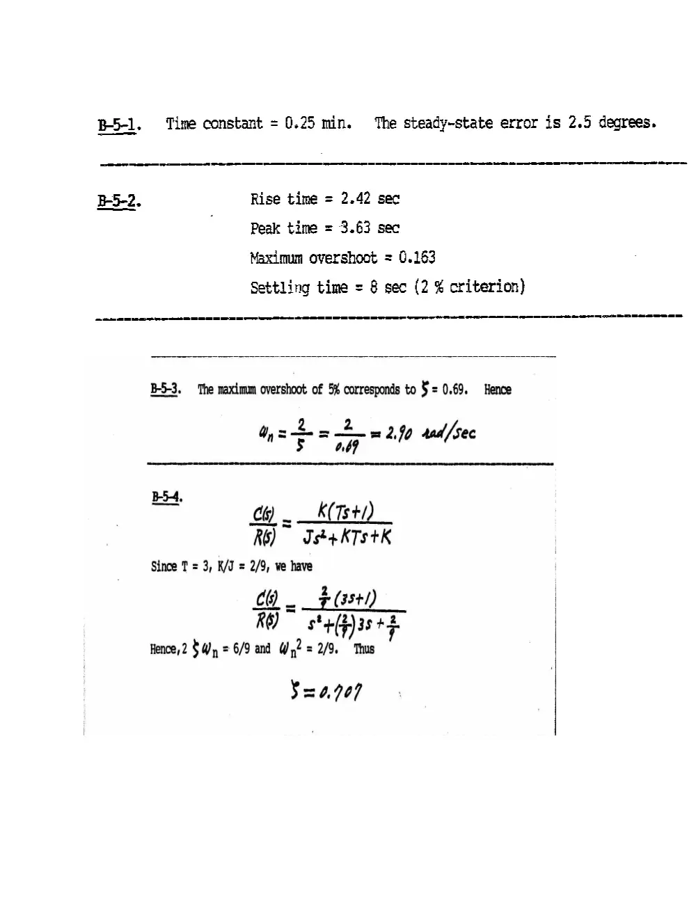
B-5-1, Time constant = 0.25 min. The steady-state error is 2.5 degrees. ar a pe Ma Sl TANS SS rere were B-5-2. Rise time = 2.42 sec Peak time = 3.63 sec Maximum overshoot = 0.163 Settling time = 8 sec (2 % criterion) i A A Po AE B-5-3. The maximm overshoot of 5% corresponds to $= 0.69. Hence 2 2 4, = = = 2, airway) 2.90 dad [sec Cy) . _K(Tst/) Ro) Ist KTS+K Since T = 3, K/J = 2/9, we have oe A) RO) s*+(4)38 +s Hence, 2 $ Wy = 6/9 and W,? = 2/9. Thus $=0.907 rr er a B-S18. For the given system we have <a K RG) St pease KAS +K Nota that Kasay = 67 = ff Since we obtain 25am - 2tkKk BXOPKRY HBtKK AR A+ GR Thus fk =e.2287 —=--__-- = — + a 5-12: % ***** Unit-step response ***** num = [0 0 10]; den =[1 2 10]; t = 0:0.02:10; step(num,den,t) gri title("Unit-Step Response’) xlabel("t Sec’) ylabel{'c(t)’) % ***** Unit-ramp response ***** - numer = [0 00 10); denr = [1 2 10 O}; c= step(numr,denr,t); plotit.e, =" tet, "=") Stle("Unit-Ramp Response’) xlabel("t Sec’) ylabel('c(t)') % ***** Unit-impulse response ***** impulse{num,den,t) gr title("Unit-impulse Response’) xlabel('t Sec’) ylabel("c(t)") 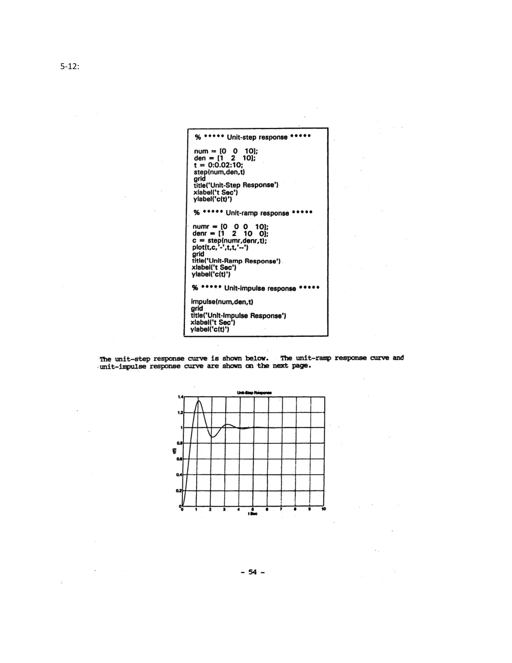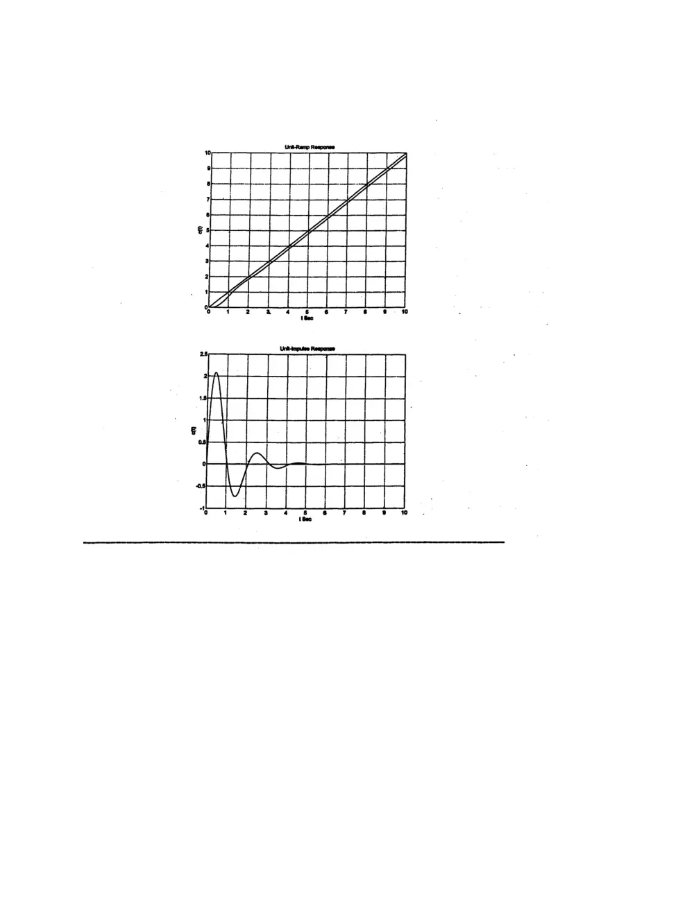The unit-step response curve is shown below. The unit-ramp response curve and -unit-impulse response curve are shown on the next page. 14