EECE 460 Homework, Spring 2007

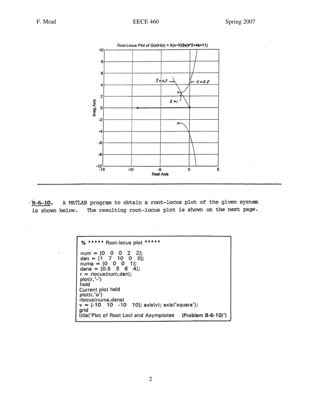
F. Mrad EECE 460 Spring 2007 Homework # 4 Solution (Exercises 6.9-10 & 15) B-6-9. The open-loop transfer function K(s+?#) GE)HE) = Sst +es+/) = 0, s=-2 + jJ7 and the zero at s = -9. The asymptotes has the poles at s = have angles + 90° and meet the reat axis at OG = 2.5. The complex branches cross the imaginary axis at s = + j 4.45. The angle of departure from the complex pole in the upper half s plane is -16.5°. The dominant closed-loop poles having the damping ratio § = 0.5 can be located as the intersection of the root loci and lines from the origin having angles + 60°. The desired dominant closed-loop poles are found to be at S=ax-“A$ tj 2.S 99 The third pole is at s = -1. The gain value corresponding to these dominant = A MATLAB program to plot the root-loci is shown Closed-loop poles is K = 1. The resulting root-locus plot is shown on the next page. below. % ***** Root-locus plot ***** num ={[0 0 1 9]; den=[1 4 11 OJ; rlocus(num,den) hold Current plot held x = [0,-3]; y = [0,5.196]; line(x,y); v={[-15 5 -10 10]; axis(v); axis('square') grid title('Root-Locus Plot of G(s)H(s) = K(s+9)/[s(s*2+4s+.11)") F. Mrad EECE 460 Spring 2007 Root-Locus Plot of G(s)H(s) = K(s+9[s(s"2+48+11) l 10 A MATLAB program to obtain a root-locus plot of the given system B6-10. 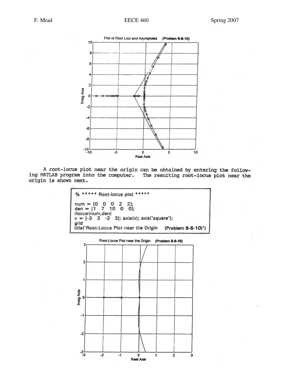The resulting root-locus plot is shown on the next page. is shown below. % ***** Root-locus plot ***** num =[0 0 O 2 2); den=[1 7 10 O OJ; numa = [0 O 0 1]; dena = [0.5 3 6 4]; r = rlocus(num,den); plot(r,'-") hold Current plot held plot(r,'o') tlocus(numa,dena) v a [-10 10 -10 10); axis(v); axis('square'); gri ; title(’Plot of Root Loci and Asymptotes (Problem B-6-10)') F. Mrad EECE 460 Spring 2007 Plot of Root Loci and Asymptotes (Problem B-€-10) | | 7 - 4 1 s 8 “196 5 0 5 10 Real Axis A root-locus plot near the origin can be obtained by entering the follow- ing MATLAB program into the computer. The resulting root~locus plot near the origin is shown next. % ***** Root-locus plot ***** num =1[0 0 O 2 2); den=[1 7 10 O QO]; tlocus(num,den) v=[-3 3 -3 3]; axis(v); axis('square’); grid title("Root-Locus Plot near the Origin (Problem B-6-10)') Root-Locus Plot near the Origin (Problem B-8-10) [TT Vit | tt | E ae a 3 0 1 2 3 Real Axis F. 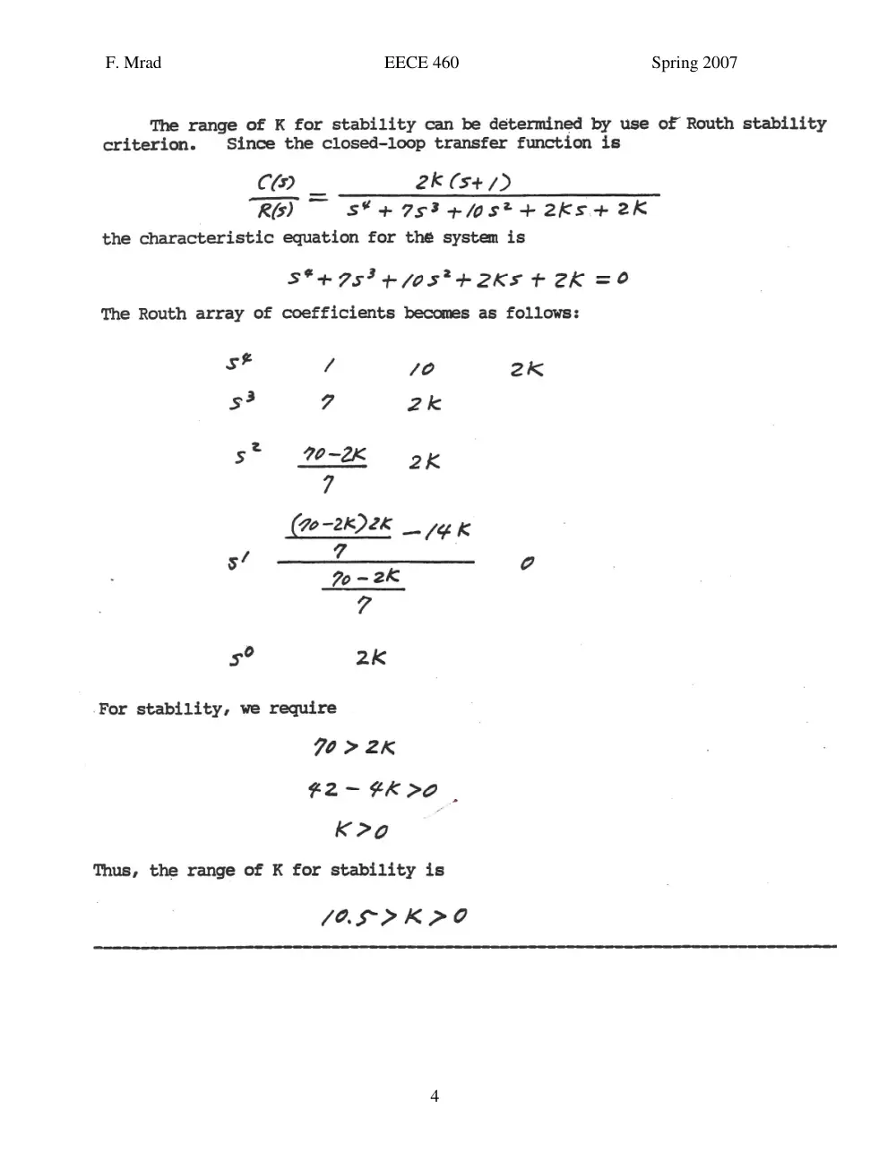Mrad EECE 460 Spring 2007 The range of K for stability can be determined by use of Routh stability criterion. Since the closed-loop transfer function is Ci) 2k (s+/)> — Rs) S%¥4+7534+/0s*+2K54+2K the characteristic equation for thé system is St47sit/os*+2Ks + 2K =O The Routh array of coefficients becomes as follows: sf / 7) 2k s? 7 2k s* 70-2K ox (2 -2K2k __ LéK Po - 2K s* 2K For stability, we require FO>2K #2-¢K>0 | K>o Thus, the range of K for stability is 108-7 K>O F. Mrad EECE 460 Spring 2007 B-6-15. The term (s + 1) in the feedforward transfer function and the term (s + 1) in the feedback transfer function cancel each other. 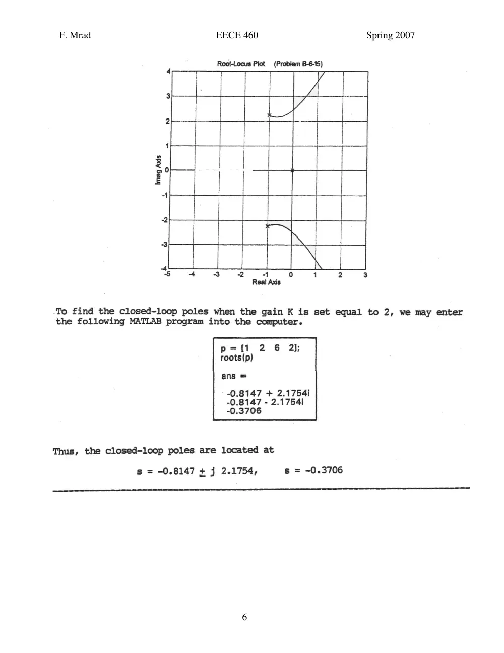The reduced characteristic equation is K(s+1) /4 kK _ S(s*2s+6) St/ ~ S(s*+ 25th) The open-loop poles of G(s)H(s) is at s=0O ands=-lt 3V5. The following MATLAB program produces the root-locus plot shown on the next page. /+ GG) = 1+ 0 % ***** Root-locus plot ***** num =[0 0 O 1]; den={1 2 6 OQ]; rlocus(num,den) Warning: Divide by zero grid [-5 3 -4 4]; axis(v); axis('square’) title("Root-Locus Plot (Problem B-6-15)") F. Mrad EECE 460 Spring 2007 Root-Locus Plot (Problem B-6-15) 4 T V | . : L __4 x | 2 1 1b g 2 — * = -4 1 2 3 > 4 « es ee | a Ke 5 4 3 2 A te) 1 2 3 Real Axis -To find the closed-loop poles when the gain K is set equal to 2, we may enter the following MATLAB program into the computer. p={[1 2 6 2j; roots(p) ans = 0.8147 + 2.1754: -0.8147 - 2.1754i -0.3706 Thus, the closed-loop poles are located at s = -0.8147 + j 2.1754, s = -0.3706 i ene nn i rer eens