
MATH 251 Notes Chapter 2, Spring 2014
American University of Beirut · Numerical Computing · 28 pages

Showing the first 10 of 28 pages. Download the PDF to see all of it.
More MATH 251 files
Show the text of this notes
CHAPTER II
Finding Roots of Real Single Valued
Functions
Nabil R. Nassif and Dolly K. Fayad
February, 2013
In this chapter we consider one of the most encountered problems in scientific computing,
which is the problem of computing the root or zero of a real-valued function f. This is
in short equivalent to computing the solution of a nonlinear equation starting from one or
several initial data , adopting some iterative method that - under favorable conditions -
will converge to a zero of the function f.
1
Introduction
Let f be a real-valued function of a real variable admitting a specific regularity on its domain
D, i.e., let f be k-times continuously differentiable, with k ≥ 1 (f ∈ Ck(D)). We seek to
find the roots of this function f, defined as follows:
Definition 1 The set R of roots of the function f(x) is defined as:
R = {r ∈ R : f(r) = 0}.
Given some computational tolerance ϵtol = 1
2101−m, m = 1, 2, ..., our objective is to compute
one or more roots of f, within such ϵtol. Specifically, for any r ∈ R, we seek an approximation
ra to r, (ra ≈ r), such that:
|r − ra|
|r|
≤ ϵtol.
(1)
(We say then, that ra approximates r up to m decimal places)
The search for a specific root of a function requires two steps.
1. Step 1: Locate the root, i.e. seek an interval (a, b), with O(|b − a|) = O(|r|), such
that:
f(x) ∈ C([a, b]), (i.e. f(x) is at least continuous)
(2)
r ∈ (a, b)
(3)
f(a) × f(b) < 0
(4)
∀ x ∈ (a, b), x ̸= r ⇒ f(x) ̸= 0
(5)
2. Step 2: Generate a sequential process leading to a sequence {rn}n≥0 the terms of which are in (a, b)
and that converges to r, i.e. satisfying:
rn ∈ (a, b) ∀ n and lim
n→∞ rn = r.
(6)
The generation of such a sequence is usually done through an iterative procedure (or
method) where rn = g(rn−1, ..., rn−k), k ≥ 1.
We start by introducing some general properties verified by such methods.
1
Definition 2 A numerical method is said to be a one-step method in case k = 1, the initial
state of the sequence being determined by the only choice of r0; otherwise, it is a multi-step
method of order k, and its initial state is then determined by the choice of r0, .., rk−1.
The order of convergence of a method measures the rate at which the sequence {rn}
generated by the numerical process converges to the root r. It is defined as follows:
Definition 3 Order of Convergence of a Method
A method is of order α > 0, if there exists a sequence of positive numbers {tn}n≥0, such that
∀n ≥ 1:
|r − rn| ≤ tn, with tn ≤ Ctα
n−1
(7)
Equivalently, in the special case where tn = |r − rn|:
|r − rn| ≤ C|r − rn−1|α
(8)
The constants C and α are independent from n, with C < 1 for n = 1.
If α = 1 the convergence is said to be linear, while if α > 1 the convergence is super-linear.
In particular, if α = 2 the convergence of the method is quadratic. (Note also that the
greatest α is, the fastest is the method.)
Definition 4 Global convergence versus Local convergence
A method is said to be globally convergent if the generated sequence {rn}n converges to r
for any choice of the initial state; otherwise it is locally convergent.
When implemented, the process generating the elements of {rn} will be stopped as soon as
the 1st computed element rn0 satisfies some predefined ”stopping criteria”.
Definition 5 Stopping criteria
Given some tolerance ϵtol, a standard stopping criterion is defined by the following relative
estimates:
|rn0 − rn0−1|
|rn0|
≤ ϵtol and |rn − rn−1|
|rn|
> ϵtol if n < n0.
(9)
The “remainder” f(rn) can also be used to set a stopping criterion since f(r) = limn→∞ f(rn) =
0. Thus, one may use a relative evaluation of the remainder. Specifically, find the first ele-
ment rn0 of the sequence {rn} satisfying:
|f(rn0)|
|f(r0)| ≤ ϵtol and |f(rn)|
|f(r0)| > ϵtol if n < n0.
(10)
2
Note also that by using the Mean-Value Theorem one has:
0 = f(r) = f(rn) + (r − rn)f ′(cn), where cn = r + θ(rn − r), θ ∈ (0, 1).
Thus if f ′ is available (referring also to (9)), a more sophisticated stopping criterion would
be:
|f(rn0)|
|rn0f ′(rn0)| ≤ ϵtol and
|f(rn)|
|rn0f ′(rn0)| > ϵtol if n < n0.
(11)
In this chapter, we shall analyze successively three root finding iterative methods: the Bi-
section method, Newton’s method and the Secant method
2
How to locate the roots of a function
There are basically two approaches to locate the roots of a function f. The first one seeks
to analyze the behaviour of f analytically or through plotting its graph, while the second
one transforms the problem of root finding into an equivalent fixed point problem. We
illustrate these methods through some specific examples.
Example 1 Locate the roots of the function f(x) = e−x − sin(x).
1. Analyzing the behaviour of the function
Since for all x < 0 the exponential e−x > 1, then one concludes that f(x) > 0.
Furthermore f(0) = 1. This implies that all the roots of the function lie in the interval
(0, ∞). Moreover, studying the variation of the function f(x) is done by studying the
sign of its derivative.
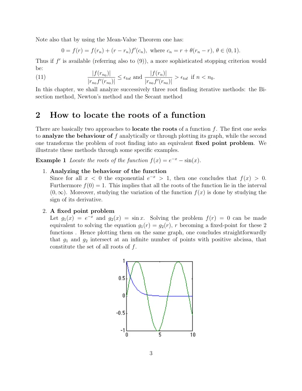
2. A fixed point problem
Let g1(x) = e−x and g2(x) = sin x.
Solving the problem f(r) = 0 can be made
equivalent to solving the equation g1(r) = g2(r), r becoming a fixed-point for these 2
functions . Hence plotting them on the same graph, one concludes straightforwardly
that g1 and g2 intersect at an infinite number of points with positive abcissa, that
constitute the set of all roots of f.
3
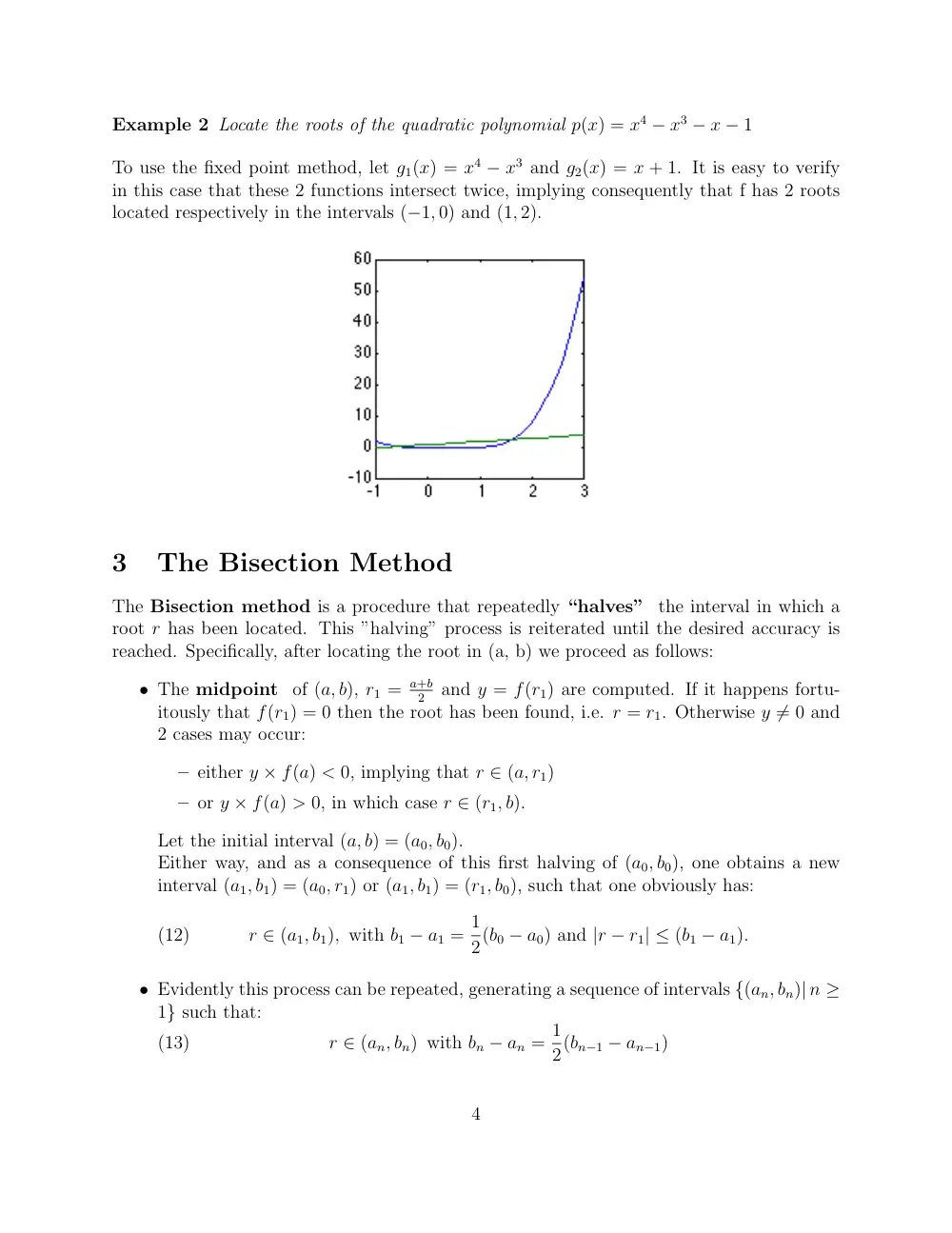
Example 2 Locate the roots of the quadratic polynomial p(x) = x4 − x3 − x − 1
To use the fixed point method, let g1(x) = x4 − x3 and g2(x) = x + 1. It is easy to verify
in this case that these 2 functions intersect twice, implying consequently that f has 2 roots
located respectively in the intervals (−1, 0) and (1, 2).
3
The Bisection Method
The Bisection method is a procedure that repeatedly “halves” the interval in which a
root r has been located. This ”halving” process is reiterated until the desired accuracy is
reached. Specifically, after locating the root in (a, b) we proceed as follows:
• The midpoint of (a, b), r1 = a+b
2
and y = f(r1) are computed. If it happens fortu-
itously that f(r1) = 0 then the root has been found, i.e. r = r1. Otherwise y ̸= 0 and
2 cases may occur:
– either y × f(a) < 0, implying that r ∈ (a, r1)
– or y × f(a) > 0, in which case r ∈ (r1, b).
Let the initial interval (a, b) = (a0, b0).
Either way, and as a consequence of this first halving of (a0, b0), one obtains a new
interval (a1, b1) = (a0, r1) or (a1, b1) = (r1, b0), such that one obviously has:
r ∈ (a1, b1), with b1 − a1 = 1
2(b0 − a0) and |r − r1| ≤ (b1 − a1).
(12)
• Evidently this process can be repeated, generating a sequence of intervals {(an, bn)| n ≥
1} such that:
r ∈ (an, bn) with bn − an = 1
2(bn−1 − an−1)
(13)
4
and a sequence of iterates {rn | n ≥ 1}, with rn ∈ (a, b) ∀n, and where
rn = 1
2(an−1 + bn−1) with |r − rn| ≤ (bn − an).
(14)
• The process is achieved when the interval (an, bn) is relatively small with respect to
the initial interval, specifically when the least value of n is reached, for which:
bn − an
b0 − a0
≤ ϵtol
(15)
where ϵtol is a given computational tolerance.
At the end of this process, the best estimate of the root r would be the last computed value
of rn as in (14).
The Bisection Method is implemented through the following algorithm:
Algorithm 1 Bisection Method
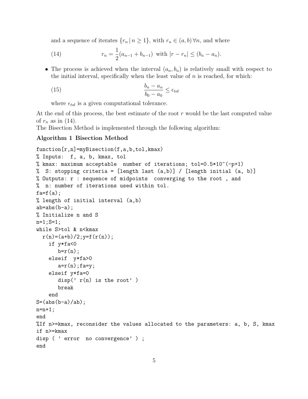
function[r,n]=myBisection(f,a,b,tol,kmax)
% Inputs:
f, a, b, kmax, tol
% kmax: maximum acceptable
number of iterations; tol=0.5*10^(-p+1)
%
S: stopping criteria = [length last (a,b)] / [length initial (a, b)]
% Outputs: r : sequence of midpoints
converging to the root , and
%
n: number of iterations used within tol.
fa=f(a);
% length of initial interval (a,b)
ab=abs(b-a);
% Initialize n and S
n=1;S=1;
while S>tol & n<kmax
r(n)=(a+b)/2;y=f(r(n));
if y*fa<0
b=r(n);
elseif
y*fa>0
a=r(n);fa=y;
elseif y*fa=0
disp(’ r(n) is the root’ )
break
end
S=(abs(b-a)/ab);
n=n+1;
end
%If n>=kmax, reconsider the values allocated to the parameters: a, b, S, kmax
if n>=kmax
disp ( ’ error
no convergence’ ) ;
end
5
The parameter kmax is used as a programming safeguard. This eliminates the possibility of
entering an infinite loop in case the sequence diverges, or also when the program is incorrectly
coded. If k exceeds kmax with bk−ak
b−a > tol, the written algorithm would then signal an error.
Thus, (12), (13) and (14) lead to the following result.
Theorem 1 Under assumptions (2)-(5), the bisection algorithm generates 2 sequences {an}n≥0
and {bn}n≥0 from which one “extracts” a sequence of iterates {rn}n≥1, with rn = an or rn =
bn, such that:
1. a0 = a, b0 = b,
2. r ∈ (an, bn)
with an < r < bn, ∀n ≥ 0,
3. The sequences {an} and {bn} are respectively monotone increasing and decreasing,
4. bn − an = bn−1−an−1
2
= b−a
2n ∀ n ≥ 1, and limn→∞ an = limn→∞ bn = r,
5. |r − rn| ≤ bn − an, ∀ n ≥ 1.
Proof. 1. and 2. are obtained by construction.
To prove 3., given (an−1, bn−1) with r ∈ (an−1, bn−1), then by definition of the method,
rn = 1
2(an−1 + bn−1) will either be an or bn. Therefore, in the case the process is reiterated,
this implies that either an = an−1 and bn < bn−1 or an > an−1 and bn = bn−1 which proves
the required result. (Note that neither of these sequences can “stagnate”. For example, the
existence of an n0 such that an0 = an, ∀n ≥ n0, would imply that r = an0, i.e. the process
is finite and the root has been found after n0 steps !).
4. follows from the “halving” procedure. It can be easily shown by induction, that bn −an =
b−a
2n and therefore limn→∞ bn − an = 0, meaning that the sequences of lengths {(bn − an)} of
the intervals {(an, bn)} converge to 0. Hence, the sequences {an} and {bn} have the same
limit point r.
Finally, to obtain 5., just note again that rn = an or bn, with r ∈ (an, bn).
A consequence of these properties is the linearity of the convergence and an estimate on
the minimum number of iterations needed to achieve a given computational tolerance ϵtol.
Specifically, we have the following result.
Corollary 1 Under the assumptions of the previous theorem, one obtains the following prop-
erties:
1. The bisection method converges linearly, in the sense of definition (3), i.e.
|r − rn| ≤ tn = bn − an, with tn ≤ 1
2tn−1
6
2. The minimum number of iterations needed to reach a tolerance of ϵtol = 0.5 × 101−p is
given by
k = ⌈(p − 1)ln(10)
ln(2) + 1⌉
Proof. The first part of the corollary is a direct result from the previous theorem. As for the
second part, it is achieved by noting that the method reaches the desired accuracy, according
to the selected stopping criteria, whenever n reaches the value k such that:
bk − ak
b − a
≤ ϵtol < bk−1 − ak−1
b − a
< ...b1 − a1
b − a = 1
2 < b0 − a0
b − a = 1.
(16)
From equation (16) and since bn−an
b−a
=
1
2n ∀ n ≥ 0, we can estimate the least number of
iterations required (theoretically) to reach the relative precision ϵtol = 1
2101−p, p being the
number of significant decimal figures fixed by the user. Such integer k satisfies then:
1
2k ≤ 1
2101−p <
1
2k−1.
(17)
Equivalently:
−k ln(2) ≤ (1 − p) ln(10) − ln(2) < −(k − 1) ln(2),
from which one concludes that:
k ln(2) ≥ (p − 1) ln(10) + ln(2) > (k − 1) ln(2),
leading to:
k ≥ (p − 1)ln(10)
ln(2) + 1 > k − 1,
(18)
The integer k is computed then as:
k = ⌈(p − 1)ln(10)
ln(2) + 1⌉.
Note that such k is independent of a and b, since it estimates the ratio bk−ak
b−a , a measure of
the relative reduction of the size of the interval (ak, bk) containing r.
The following table provides values of k relative to a fixed precision p.
precision p
Iterations k
3
8
5
15
7
21
10
31
15
48
7
Obviously the method is slowly convergent ! Nevertheless, since at each step the length of
the interval is reduced by a factor of 2, it is advantageous to choose the initial interval as
small as possible.
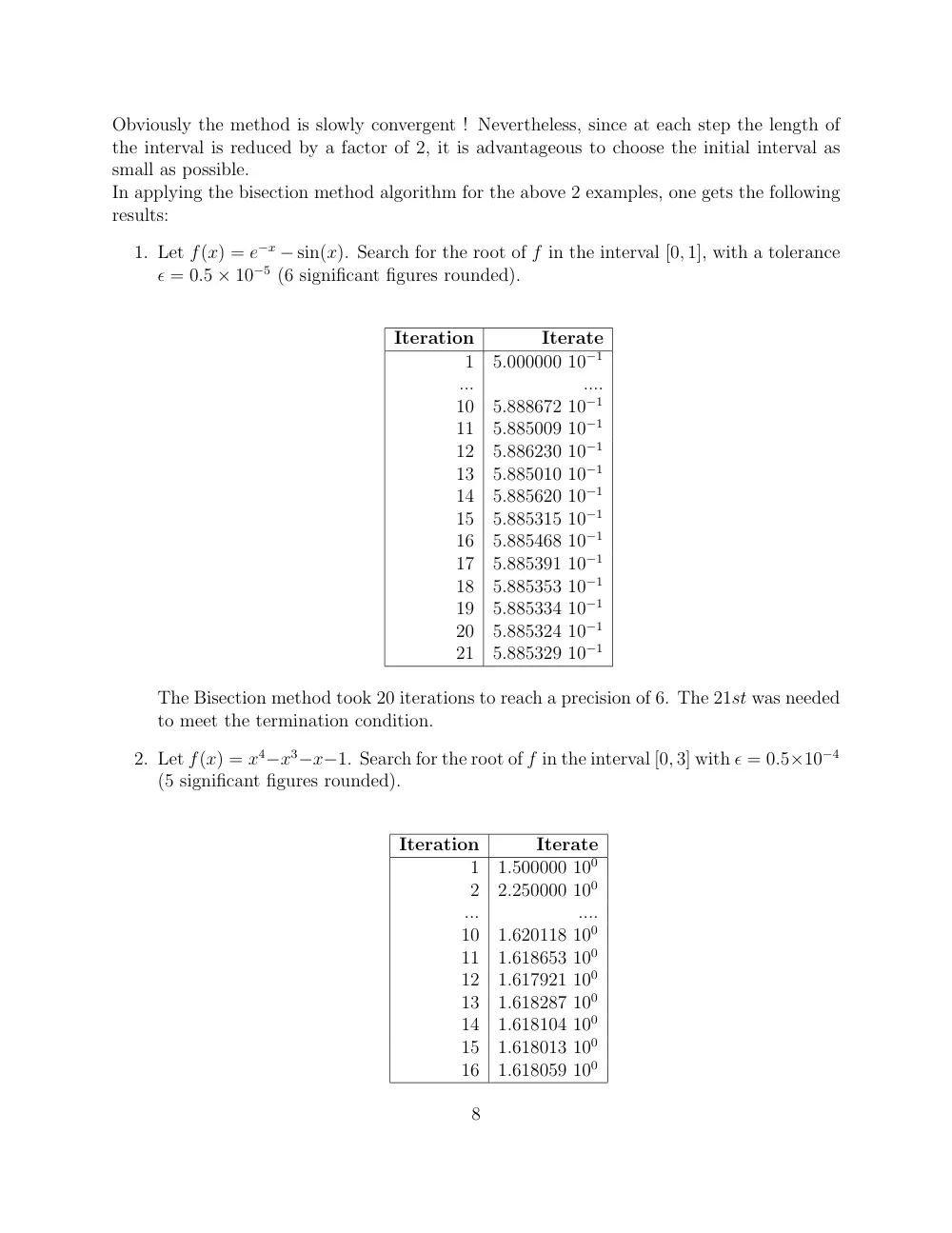
In applying the bisection method algorithm for the above 2 examples, one gets the following
results:
1. Let f(x) = e−x − sin(x). Search for the root of f in the interval [0, 1], with a tolerance
ϵ = 0.5 × 10⁻⁵ (6 significant figures rounded).
Iteration
Iterate
1
5.000000 10−1
...
....
10
5.888672 10−1
11
5.885009 10−1
12
5.886230 10−1
13
5.885010 10−1
14
5.885620 10−1
15
5.885315 10−1
16
5.885468 10−1
17
5.885391 10−1
18
5.885353 10−1
19
5.885334 10−1
20
5.885324 10−1
21
5.885329 10−1
The Bisection method took 20 iterations to reach a precision of 6. The 21st was needed
to meet the termination condition.
2. Let f(x) = x4−x3−x−1. Search for the root of f in the interval [0, 3] with ϵ = 0.5×10⁻⁴
(5 significant figures rounded).
Iteration
Iterate
1
1.500000 100
2
2.250000 100
...
....
10
1.620118 100
11
1.618653 100
12
1.617921 100
13
1.618287 100
14
1.618104 100
15
1.618013 100
16
1.618059 100
8
To conclude, the Bisection is a multi-step method that, although conceptually clear and
simple, has significant drawbacks since it is relatively slow. However it globally converges
to the searched solution and is often used as a starter for other more efficient locally con-
vergent methods, notably both Newton’s and Secant methods.
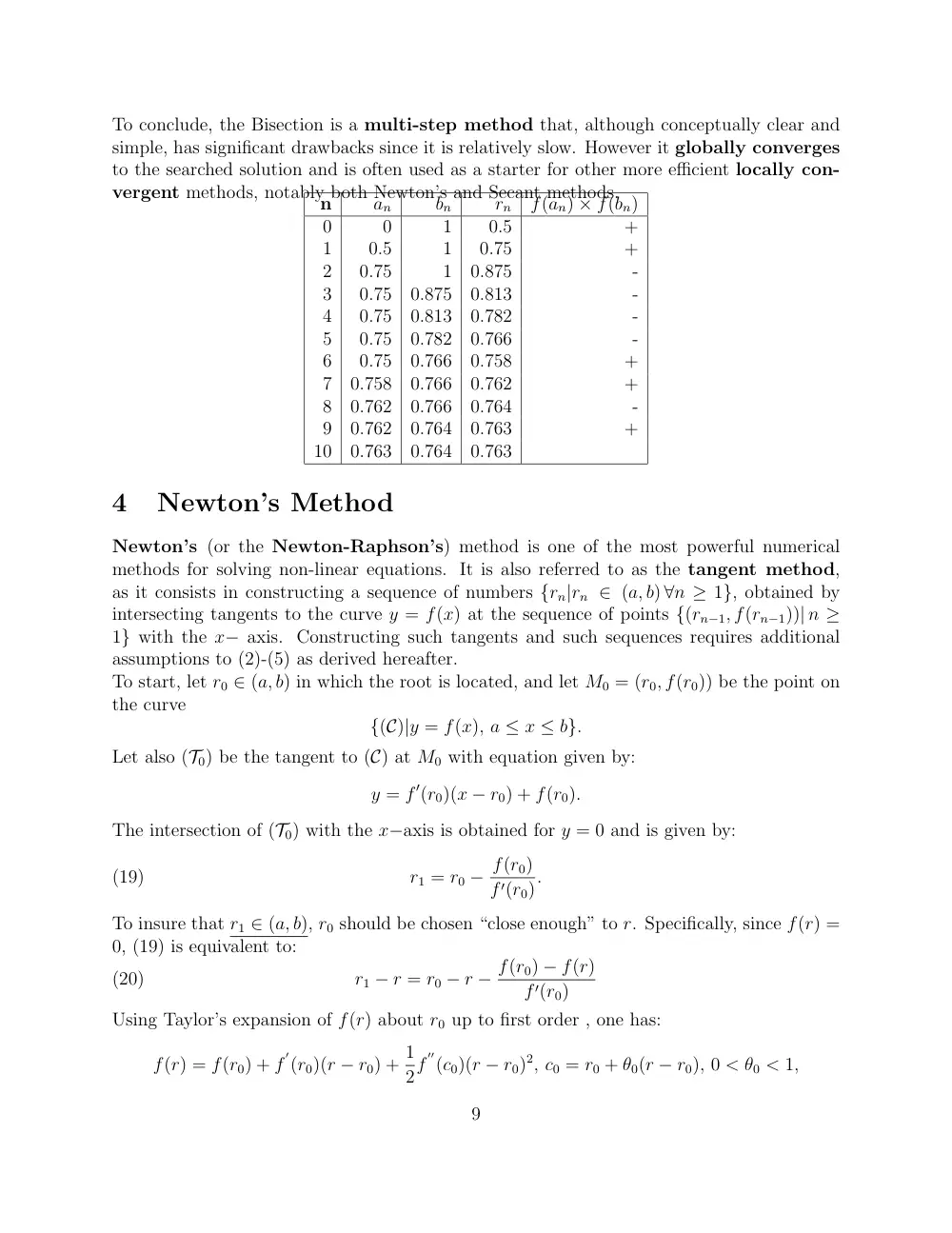
n
an
bn
rn
f(an) × f(bn)
0
0
1
0.5
+
1
0.5
1
0.75
+
2
0.75
1
0.875
-
3
0.75
0.875
0.813
-
4
0.75
0.813
0.782
-
5
0.75
0.782
0.766
-
6
0.75
0.766
0.758
+
7
0.758
0.766
0.762
+
8
0.762
0.766
0.764
-
9
0.762
0.764
0.763
+
10
0.763
0.764
0.763
4
Newton’s Method
Newton’s (or the Newton-Raphson’s) method is one of the most powerful numerical
methods for solving non-linear equations. It is also referred to as the tangent method,
as it consists in constructing a sequence of numbers {rn|rn ∈ (a, b) ∀n ≥ 1}, obtained by
intersecting tangents to the curve y = f(x) at the sequence of points {(rn−1, f(rn−1))| n ≥
1} with the x− axis. Constructing such tangents and such sequences requires additional
assumptions to (2)-(5) as derived hereafter.
To start, let r0 ∈ (a, b) in which the root is located, and let M0 = (r0, f(r0)) be the point on
the curve
{(C)|y = f(x), a ≤ x ≤ b}.
Let also (T0) be the tangent to (C) at M0 with equation given by:
y = f ′(r0)(x − r0) + f(r0).
The intersection of (T0) with the x−axis is obtained for y = 0 and is given by:
r1 = r0 − f(r0)
f ′(r0).
(19)
To insure that r1 ∈ (a, b), r0 should be chosen “close enough” to r. Specifically, since f(r) =
0, (19) is equivalent to:
r1 − r = r0 − r − f(r0) − f(r)
f ′(r0)
(20)
Using Taylor’s expansion of f(r) about r0 up to first order , one has:
f(r) = f(r0) + f
′(r0)(r − r0) + 1
2f
′′(c0)(r − r0)2, c0 = r0 + θ0(r − r0), 0 < θ0 < 1,
9
thus leading to:
f(r) − f(r0)
f
′(r0)
= (r − r0) + 1
2
f
′′(c0)
f
′(r0) (r − r0)2, with c0 ∈ (a, b).
Hence, imposing on f and on the interval (a, b) the following additional assumptions:
f(x) ∈ C2(a, b), i.e. f(x), f
′(x), f
′′(x) are continuous on (a, b)
(21)
f
′(x) ̸= 0 ∀ x ∈ (a, b)
(22)
ones concludes from (20):
|r1 − r| = 1
2
|f
′′(c0)|
|f
′(r0)| (r − r0)2
(23)
Based on these additional assumptions, we define also the positive constant:
C = 1
2
maxx∈(a,b) |f
′′(x)|
minx∈(a,b) |f
′(x)| .
(24)
which will then lead to:
|r − r1| ≤ C|r − r0|2
(25)
This gives a preliminary ”closeness” result of r1 with respect to the root r, in terms of the
”closeness” of r0, without however insuring yet the required location of r1 in (a, b). In this
view, letting now:
I0 = {x| |r − x| < 1
C } ∩ (a, b)
(26)
and selecting initially r0 in I0, leads to the required result as shown hereafter.
Lemma 1 If r0 ∈ I0 as defined in (26), then r1 ∈ I0 with
|r − r1| ≤ |r − r0|
(27)
Proof.
Let ei = C|r − ri|, i = 0, 1, where C verifies (24).
Multiplying (25) by C one
obviously has:
e1 ≤ e2
0
moreover, since e0 < 1 and C > 0, the required result is reached.
Thus selecting r0 ∈ I0 and reaching r1 satisfying (27 ), the process can be continued be-
yond that step. In fact one generates a sequence of Newton’s iterates {rn| n ≥ 2} with
rn ∈ (a, b) ∀ n, given by a formula generalizing (19). Specifically, one has:
rn+1 = rn − f(rn)
f ′(rn), n ≥ 0.
(28)
with (rn+1, 0) being the intersection with the x-axis of the tangent to the curve (C) at the
point (rn, f(rn)).
10
Clearly, Newton’s method is a one-step iteration rn+1 = g(rn), with the iteration function
g(x) given by:
g(x) = x − f(x)
f ′(x).
(29)
We turn now to the analysis of the convergence of Newton’s method, i.e. the convergence of
Newton’s iterates {rn}n≥0.
Theorem 2 Let f(x) satisfies assumptions (2)-(5), in addition to (21) and (22), then for
r0 ∈ I0, with C as defined in (24), the sequence of Newton’s iterates:
rn+1 = rn − f(rn)
f ′(rn), n ≥ 0,
is such that:
1. rn ∈ I0, ∀n ≥ 0
2. limn→∞ rn = r
3. |r − rn+1| ≤ C|r − rn|2, meaning that Newton’s method is quadratic with α = 2.
Proof. The proof of this theorem follows from arguments used to obtain lemma 1. In fact,
one derives as for (25) that:
en+1 ≤ e2
n, ∀n ≥ 0.
(30)
where ei = C|r − ri|, i = n, n + 1.
Moreover, it can be easily proved by induction on n, that (30 ) in turn implies that:
en ≤ (e0)2n ∀ n ≥ 1.
(31)
As e0 < 1 then rn ∈ I0 with limn→∞ en = 0, proving parts 1 and 2 of the lemma. In addition
to these results, and as derived in (23) and (25), one concludes that :
|rn+1 − r| = 1
2
|f
′′(cn)|
|f
′(rn)| (r − rn)2 ≤ C|r − rn|2,
(32)
11
with cn = rn + θn(r − rn), 0 < θn < 1. Referring to (8) that result obviously implies that
α = 2,
Note also that inequality (31) allows obtaining an estimate on the minimum number of
iterations needed to reach a computational tolerance ϵtol = 0.5 × 101−p . Specifically, we
prove now:
Corollary 2 If r0 ∈ I0, the minimum number of iterations needed to reach ϵtol = 0.5×101−p
is given by:
n0 = ⌈ ln(1 + (p − 1) ln(10) + ln(2)
| ln(e0)|
)/ ln(2)⌉.
Proof. Note that ϵtol is reached whenever n = n0 satisfies the following inequalities:
|r − rn0|
|r − r0| ≤ 0.5 × 101−p < |r − rn|
|r − r0|, ∀ n < n0,
Since also |r−rn|
|r−r0| = en
e0 , ∀n ≥ 1, then from (31):
|r − rn0|
|r − r0| ≤ (e0)2n0−1.
The sought for minimum number of iterations n0 would thus verify:
(e0)2n0−1 ≤ 0.5 × 101−p < (e0)2n−1, ∀ n < n0.
Since e0 < 1, this is equivalent to:
2n0 ≥ 1 + (p − 1) ln(10) + ln(2)
| ln(e0)|
> 2n, n < n0.
This leads to n0 satifying:
n0 ≥
ln(1 + (p−1) ln(10)+ln(2)
| ln(e0)|
)
ln(2)
> n0 − 1
and therefore:
n0 = ⌈ ln(1 + (p − 1) ln(10) + ln(2)
| ln(e0)|
)/ ln(2)⌉,
which is the desired result.
To illustrate, assume e0 = 1
2, then it results from this lemma that:
n0 = ⌈ ln(2 + (p − 1)ln(10)
ln(2) )/ ln(2)⌉.
The following table provides values of n0 relative to a precision p.
12
precision p
Iterations n0
7
4
10
5
16
6
Thus, one can assert that Newton’s method is a locally and quadratically convergent
method. When a root r of a function f(x) is located in an interval (a, b), the first step is to
insure finding a sub-interval I0 ⊂ (a, b) containing r, in which |r−r0| ≤ 1
C, with the constant
C given in (24).
A rule of thumb would be to select r0 after 1 or 2 applications of the bisection method. Such
a step would make sure the initial condition r0 is close “enough” to r.
The following example illustrates the general behavior of Newton’s method.
Example 3 Find the roots of f(x) = sin(x) − e−x in the interval (0, 2), using Newton’s
method.
Obviously, Newton’s method is not applicable when the initial choice of the iteration r0 is
selected from the whole interval (0, 2). For example if r0 is chosen in the interval (1.5, 2),
the generated sequence {rn} may not fall in the interval (0, 2) and thus fails to converge,
as is shown in the following table resulting from the application of Newton’s algorithm with
r0 = 1.75.
Iteration
Iterate
0
1.75
1
1.8291987×10²
2
1.8206468×10²
3
1.8221346×10²
4
1.8221237×10²
...
...
Obviously, the convergence is taking place to a root that is not in the interval (0, 2). On the
other hand, one application of the bisection method would start the iteration with r0 = 1,
leading to the following efficiently convergent process.
13
Iteration
Iterate
0
1.0
1
4.785277889803116×10⁻¹
2
5.841570194114709×10⁻¹
3
5.885251122073911×10⁻¹
4
5.885327439585476×10⁻¹
5
5.885327439818611×10⁻¹
6
5.885327439818611×10⁻¹
Obviously, about 4 iterations would provide 10 significant figures, a fifth one leading to 16
figures, i.e. a more than a double precision answer.
However, there are cases, as in the first Example below, where the convergence of the method
is not affected by the choice of the initial condition, whereby Newton’s method converges
unconditionally.
Example 4 The square root function
Using Newton’s method, we seek an approximation to r = √a, where a > 0..
Clearly, such r is the unique positive root of f(x) = x2 −a, with Newton’s iterates satisfying
the following identity:
rn+1 = rn − f(rn)
f ′(rn) ≡ 1
2(rn + a
rn
), ∀ n ≥ 0
(33)
(It is easy to check graphically that the sequence converge to √a for any initial choice of
r0 > 0).
Based on the equation above:
rn+1 − r = 1
2(rn − 2r + a
rn
)
Equivalently, since a = r2 :
rn+1 − r = (rn − r)2
2rn
≥ 0
(34)
The following results can therefore be deduced:
1. rn ≥ r, ∀ n ≥ 1
2. The generated iterative sequence {rn} is a decreasing sequence, since:
rn+1 − rn = − f(rn)
f ′(rn) = −(r2
n − r2)
2rn
≤ 0
based on the property 1. above.
14
3. The sequence {rn} converges to the root of f, i.e. limn→∞ rn = r, since rewriting (34)
as:
rn+1 − r = rn − r
2
(1 − r
rn
)
in turn by induction leads to:
rn+1 − r < 1
2(rn − r) < ... <
1
2(n−1)(r1 − r)
4. The convergence is notably quadratic, since from (34) and for all n ≥ 0:
|rn+1 − r| = |(rn − r)2
2rn
| < C|rn − r|2 where C = 1
2r
As for IEEE standard notations, note that since
a = m × 2e with 1 ≤ m < 2
then the square root function is such that:
√ : (m, e) → (m′, e′) with √a = m′ × 2e′
The normalized mantissa and exponent of √a are computed as follows:
1. if e = 2k, then m′ = √m with 1 ≤ m′ <
√
2 < 2, and e′ = k, i.e.
√ : (m, e = 2k) → (m′ = √m, e′ = k)
2. if e = 2k + 1, then a = 2m × 22k and m′ =
√
2m with 1 <
√
2 ≤ m′ < 2, and e′ = k,
i.e.
√ : (m, e = 2k + 1) → (m′ =
√
2m, e′ = k)
In either case, Newton’s iteration in binary mode may start with r0 = 1.
The local character of convergence of Newton’s method is well illustrated in the interest-
ing case of the reciprocal function.
Example 5 The reciprocal of a positive number function
Assume a > 0. We seek an approximation to r = 1
a, where r is the unique positive root of
f(x) = a − 1
x. Obviously, Newton’s iterations satisfy the following identity:
rn+1 = rn(2 − arn), ∀ n ≥ 0
(35)
Choosing restrictively the initial condition r0 ∈ (0, 2/a) leads to an iterative sequence {rn}
where:
rn+1 > 0, whenever rn ∈ (0, 2/a)
(36)
In such case, for all n ≥ 1, it is left as an exercise to prove that:
15
1. rn+1 − r = − (rn−r)2
r
2. The generated sequence is an increasing sequence
3. The sequence {rn} converges to the root of f, i.e. limn→∞ rn = r
4. Convergence of the sequence is quadratic.
Considering IEEE standard notations as for the square root function example, if
a = m × 2e , with 1 < m < 2
then the inverse function is such that:
inv : (m, e) → (m′, e′), with 1
a = m′ × 2e′
The normalized mantissa and exponent of 1/a are respectively:
m′ = 2/m and e′ = −e − 1
since 1
a = 1
m × 2−e or more adequately:
1
a = 2
m × 2−e−1, with 1 < 2
m < 2
5
The Secant Method
Recall that Newton’s iteration satisfies formula (28):
rn+1 = rn − f(rn)
f ′(rn) where f ′(rn) = lim
h→0
f(rn + h) − f(rn)
h
One drawback of Newton’s method is the necessary availability of the derivative. In case
such function is difficult to program, an alternative would be to avoid the calculation of
f ′(rn), and replace it by the backward divided difference approximation to the derivative:
f ′(rn) ≈ [rn−1, rn] = f(rn) − f(rn−1)
rn − rn−1
This would suggest obtaining rn+1 using the secant to the curve y = f(x) passing through
the points (rn−1, f(rn−1)) and (rn, f(rn)), the equation of which is:
y = f(rn) − f(rn−1)
rn − rn−1
(x − rn) + f(rn)
16
The intersection of this secant line with the x− axis would provide the (n+1)-iterate secant
method formula:
rn+1 = rn −
f(rn)
[rn, rn−1] ≡ rn − f(rn)(rn − rn−1)
f(rn) − f(rn−1) , n ≥ 2
(37)
The secant method is a two-steps method of the form rn+1 = g(rn, rn−1), its processing
requiring selection of r0 and r1. Of course, if the method is succeeding, the points rn will be
approaching a zero of f, so f(rn) will be converging to zero.
Practically, if a root r of the function f is located in the interval (a, b), one would suggest
applying twice the bisection method in order to implement (37) as shown in the following
algorithm.
Algorithm 2 Secant Method
% Input f, a, b,TOL, kMAX
% Find the first 2 approximations by the ‘‘Bisection rule"
function[r,k]=mySecant(f,a,b,TOL,kmax)
r(1)=(a+b)/2 ;
if f(a)*f(r(1)) < 0
r(2)=(r(1)+a)/2 ;
else
r(2)=(b+r(1))/2 ;
end
k=2; S = 1;
while S >TOL & k<=kMAX
d=(f(r(k))-f(r(k-1))/r(k)-r(k-1));
r(k+1)=r(k)-f(r(k))/d;
S = abs (r(k+1)-r(k)])
abs (r(k)) ;
k=k+1;
end
17
The advantages of the secant method relative to the tangent method are that (after the first
step) only one function evaluation is required per step (in contrast to Newton’s iteration
which requires 2) and that it is almost as rapidly convergent. It can be shown that under
the same assumptions as those of Theorem 2 , the basic secant method is superlinear and
has a local character of convergence.
Theorem 3 Under the hypothesis of Theorem 2 and for r0 and r1 ∈ I0 (defined in (26)),
then one has:
1. limn→∞ rn = r,
2. There exists a sequence {tn|, n ≥ 0} such that:
|r − rn| ≤ tn, with tn = O(tn−1)γ and γ = 1 +
√
5
2
(38)
i.e the order of convergence
of the secant method is the Golden Number γ ≈
1.618034 in the sense of (7).
Proof. Starting with the following identity (Theorem 4.5) :
f(r) = f(rn) + [rn−1, rn](r − rn) + 1
2(r − rn)(r − rn−1)f ′′(c) ; c = rn + θ(r − rn), 0 < θ < 1
where f(r) = 0, one deduces:
rn −
f(rn)
[rn−1, rn] = r + 1
2(r − rn)(r − rn−1)
f”(c)
[rn−1, rn]
Since [rn−1, rn] = f ′(c1), then under the assumptions of Theorem 2 , one concludes that:
|r − rn| ≤ C|r − rn−1|.|r − rn−2|, ∀n ≥ 2
(39)
with C as defined in (24). Again, let ei = C|r − ri|, i = n − 2, n − 1, then (39) is equivalent
to:
en ≤ en−1.en−2, ∀n ≥ 2.
(40)
With the assumption that the initial conditions r0, r1 are selected so that:
δ = max(e0, e1) < 1
(41)
one obviously concludes that e2 ≤ e0e1 < δ2 and that e3 ≤ e1e2 < δ3. Let {fn|n ≥ 0} be a
Fibonacci sequence defined by:
f0 = f1 = 1, fn = fn−1 + fn−2, n ≥ 2.
18
It is well known that the solution of this second order difference equation is given by:
fn = 1
√
5((1 +
√
5
2
)n+1 − (1 −
√
5
2
)n+1) = 1
√
5((1 +
√
5
2
)n+1 + (−1)n+1(
√
5 − 1
2
)n+1).
Let γ = 1+
√
5
2
be the Golden Number, then:
fn = 1
√
5(γn+1 + (−1
γ )n+1)
As n → ∞, the first term of fn tends to +∞ while the second tends to 0 so that fn = O(γn+1).
Based on the choice of r0 and r1 in I0, e0 < δf0 and e1 < δf1. By induction, assuming that
ek < δfk, ∀k ≤ n − 1, then using (40), one has:
en ≤ en−1en−2 < δfn−1+fn−2 = δfn, ∀n ≥ 2.
(42)
As δ < 1, this last inequality proves the first part of the theorem, i.e. that
lim
n→∞ en = 0.
As for the second part of the theorem, given that:
|r − rn| ≤ 1
C en < tn = 1
C δfn,
then:
tn
tγ
n−1
= Cγ−1δfn−γfn−1.
Note that
fn − γfn−1 = 1
√
5(γn+1 + (−1
γ )n+1 − γn+1 − γ(−1
γ )n) = 2
√
5(−1
γ )n+1.
Hence fn − γfn−1 → 0 and therefore there exist a constant K such that:
tn ≤ K(tn−1)γ.
To illustrate the Secant method, we consider the following example.
Example 6 Approximate the root of f(x) = sin x − e−x up to 10 decimal figures, in the
interval (0, 2) using the Secant’s method.
This process gives the following results:
19
Iteration
Iterate
0
1.0
1
1.5000000000
2
0.21271008648
3
0.77325832517
4
0.61403684201
5
0.58643504642
6
0.58855440366
7
0.58853274398
8
0.58853274398
Besides computing the initial conditions, the Secant ’s method requires about 6 iterations
to reach a precision p = 10, that is 2 more than Newton’s method.
Comparisons between the convergence of both Newton and Secant methods can be further
made, using the inequalities (31) and (42), as en = C|r − rn| satisfies respectively:
1. en ≤ δ2n in Newton’s method and
2. en ≤ δfn in the secant method.
with δ = e0 = C|r − r0|. Thus
|r − rn|
|r − r0| = en
e0
=≤ δ2n−1
for Newton’s method and
|r − rn|
|r − r0| = en
e0
=≤ δfn−1
for the secant method.
In the same way that this was done for the preceding methods (Corollaries 1 and 2), one
can also derive the minimum number of iterations needed theoretically to reach requested
precisions using the secant method. However in this chapter, in order to confirm that New-
ton’s method is faster, we will only consider for example the specific case of δ = 1
2, seek-
ing the minimum n0 for which |r−rn|
|r−r0| ≤ 2−p, (i.e a precision p in a floating-point system
F(2, p, Emin, Emax)). Straightforward it can be shown that such n0 satisfies:
2n(1)
0
≥ 1 + p > 2n(1)
0 −1
for Newton’s method and
fn(2)
0
≥ 1 + p > fn(2)
0 −1
for the secant method. We summarize the results in the following table:
20
p
n(1)
0
n(2)
0
10
4
6
24 (IEEE-single)
5
8
53 (IEEE-double)
6
9
Thus although Newton’s method is faster, it takes at most about 2 to 3 more iterations for
the secant method to reach a same precision.
21
6
Exercises
The Bisection Method
1. Locate all the roots of f, then approximate each one of them up to 3 decimal figures
using the Bisection method.
(a) f(x) = x − 2 sin x
(b) f(x) = x3 − 2 sin x
(c) f(x) = ex − x2 + 4x + 3
(d) f(x) = x3 − 5x − x2
2. Show that the following equations have infinitely many roots by graphical methods.
Use the Bisection method to determine the smallest positive value up to 4 decimal
figures.
(a) tan x = x
(b) sin x = e−x
(c) cos x = ex
(d) ln(x + 1) = tan(2x)
3. The following functions have a unique root in the interval [1, 2]. Use the Bisection
method to approximate that root up to 3 decimal figures. Compare the number of
iterations needed to reach that precision with the predictable “theoretical” value.
(a) f(x) = x3 − ex
(b) f(x) = x2 − 4x + 4 − ln x
(c) f(x) = x3 + 4x2 − 10
(d) f(x) = x4 − x3 − x − 1
(e) f(x) = x5 − x3 + 3
(f) f(x) = e−x − cos x
(g) f(x) = ln(1 + x) −
1
x+1
4. The following functions have a unique root in the interval [0, 1]. Use the Bisection
method to approximate that root up to 5 decimal figures. Compare the number of
iterations needed to reach that precision with the predictable “theoretical” value.