MATH 251 Notes Chapter 5, Spring 2014

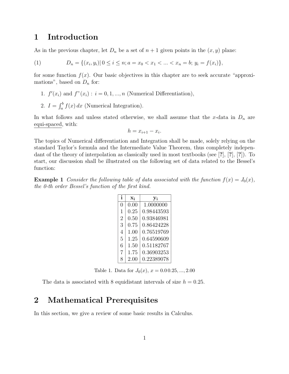
CHAPTER V NUMERICAL DIFFERENTIATION AND INTEGRATION Nabil R. Nassif and Dolly K. Fayad April 2012 1 Introduction As in the previous chapter, let Dn be a set of n + 1 given points in the (x, y) plane: Dn = {(xi, yi)| 0 ≤ i ≤ n; a = x0 < x1 < ... < xn = b; yi = f(xi)}, (1) for some function f(x). Our basic objectives in this chapter are to seek accurate “approxi- mations”, based on Dn for: 1. f ′(xi) and f”(xi) : i = 0, 1, ..., n (Numerical Differentiation), 2. I = � b a f(x) dx (Numerical Integration). In what follows and unless stated otherwise, we shall assume that the x-data in Dn are equi-spaced, with: h = xi+1 − xi. The topics of Numerical differentiation and Integration shall be made, solely relying on the standard Taylor’s formula and the Intermediate Value Theorem, thus completely indepen- dant of the theory of interpolation as classically used in most textbooks (see [?], [?], [?]). To start, our discussion shall be illustrated on the following set of data related to the Bessel’s function: Example 1 Consider the following table of data associated with the function f(x) = J0(x), the 0-th order Bessel’s function of the first kind. i xi yi 0 0.00 1.0000000 1 0.25 0.98443593 2 0.50 0.93846981 3 0.75 0.86424228 4 1.00 0.76519769 5 1.25 0.64590609 6 1.50 0.51182767 7 1.75 0.36903253 8 2.00 0.22389078 Table 1. Data for J0(x), x = 0.0 0.25, ..., 2.00 The data is associated with 8 equidistant intervals of size h = 0.25. 2 Mathematical Prerequisites In this section, we give a review of some basic results in Calculus. 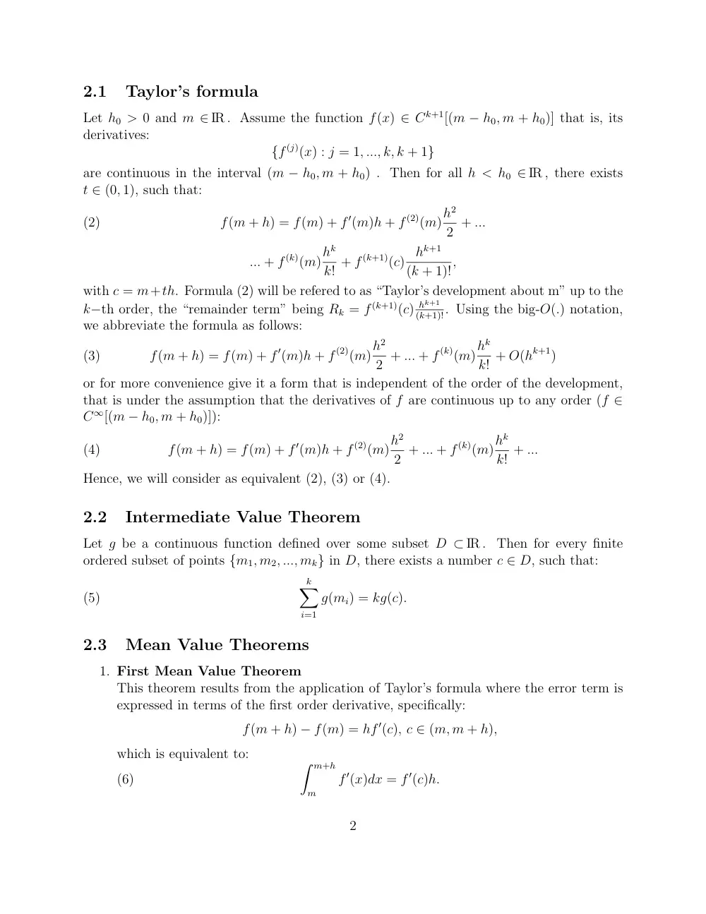1 2.1 Taylor’s formula Let h0 > 0 and m ∈ IR . Assume the function f(x) ∈ Ck+1[(m − h0, m + h0)] that is, its derivatives: {f (j)(x) : j = 1, ..., k, k + 1} are continuous in the interval (m − h0, m + h0) . Then for all h < h0 ∈ IR , there exists t ∈ (0, 1), such that: f(m + h) = f(m) + f ′(m)h + f (2)(m)h2 2 + ... (2) ... + f (k)(m)hk k! + f (k+1)(c) hk+1 (k + 1)!, with c = m+th. Formula (2) will be refered to as “Taylor’s development about m” up to the k−th order, the “remainder term” being Rk = f (k+1)(c) hk+1 (k+1)!. Using the big-O(.) notation, we abbreviate the formula as follows: f(m + h) = f(m) + f ′(m)h + f (2)(m)h2 2 + ... + f (k)(m)hk k! + O(hk+1) (3) or for more convenience give it a form that is independent of the order of the development, that is under the assumption that the derivatives of f are continuous up to any order (f ∈ C∞[(m − h0, m + h0)]): f(m + h) = f(m) + f ′(m)h + f (2)(m)h2 2 + ... + f (k)(m)hk k! + ... (4) Hence, we will consider as equivalent (2), (3) or (4). 2.2 Intermediate Value Theorem Let g be a continuous function defined over some subset D ⊂ IR . Then for every finite ordered subset of points {m1, m2, ..., mk} in D, there exists a number c ∈ D, such that: k � i=1 g(mi) = kg(c). (5) 2.3 Mean Value Theorems 1. First Mean Value Theorem This theorem results from the application of Taylor’s formula where the error term is expressed in terms of the first order derivative, specifically: f(m + h) − f(m) = hf ′(c), c ∈ (m, m + h), which is equivalent to: � m+h m f ′(x)dx = f ′(c)h. (6) 2 2. Second Mean Value Theorem This one generalizes the previous one, (6) becoming: � m+h m w(x)g(x)dx = g(c) � m+h m w(x)dx, (7) where g(x) and w(x) are continuous functions with w(x) ≥ 0 (or w(x) ≤ 0). 3 Numerical Differentiation 3.1 1st order Derivatives and Divided Differences Based on the set of points (1), Divided Differences appear to provide efficient “discrete” tools to approximate derivatives. This is illustrated by the following proposition which is essential in this chapter. Theorem 1 Assume that the function f is k-times continuously differentiable in D. Then for every subset of distinct points {xi, xi+1, ..., xi+k} in D, there exists c ∈ (xi, xi+k), such that [xi, xi+1, ..., xi+k] = f (k)(c) k! . 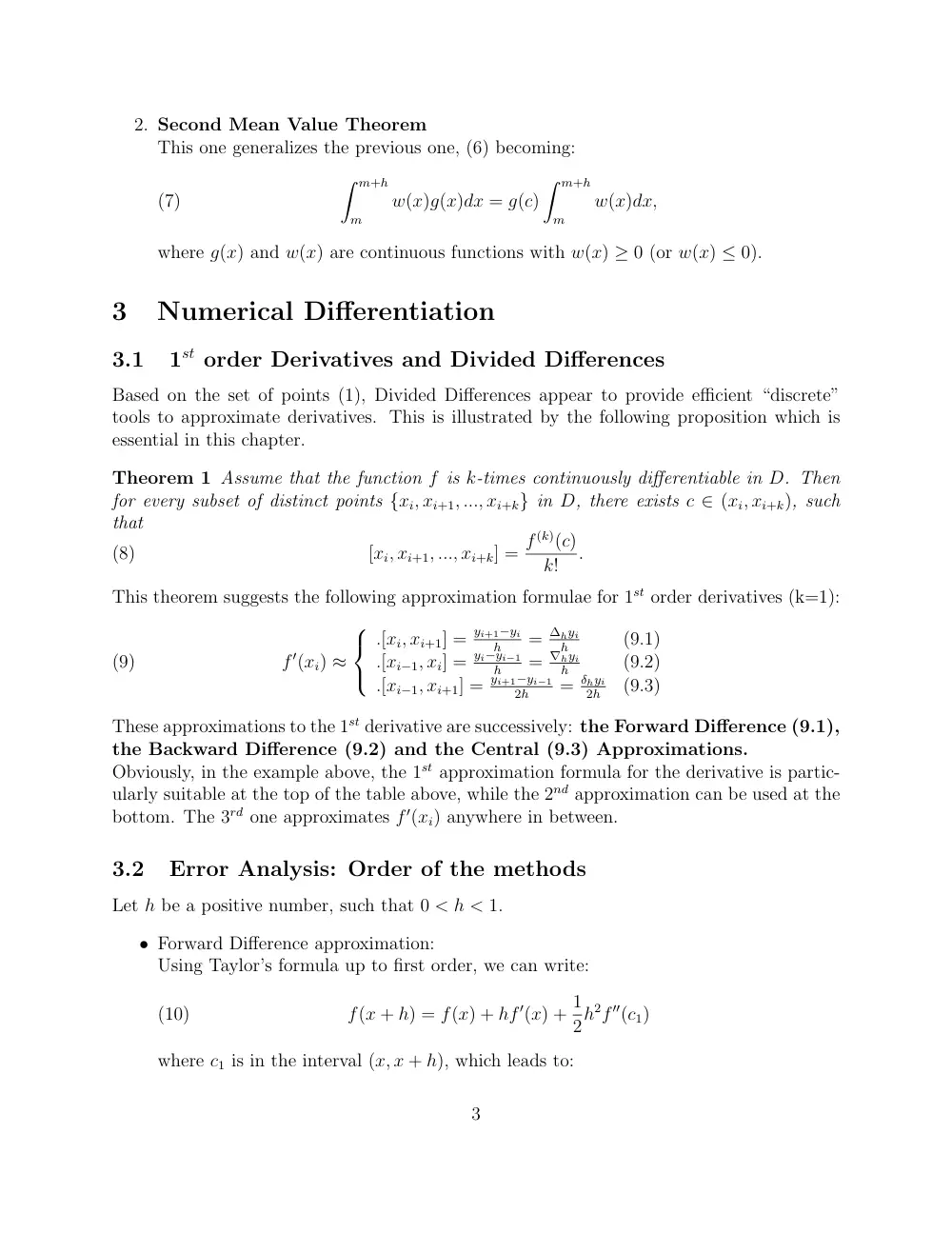(8) This theorem suggests the following approximation formulae for 1st order derivatives (k=1): f ′(xi) ≈    .[xi, xi+1] = yi+1−yi h = ∆hyi h (9.1) .[xi−1, xi] = yi−yi−1 h = ∇hyi h (9.2) .[xi−1, xi+1] = yi+1−yi−1 2h = δhyi 2h (9.3) (9) These approximations to the 1st derivative are successively: the Forward Difference (9.1), the Backward Difference (9.2) and the Central (9.3) Approximations. Obviously, in the example above, the 1st approximation formula for the derivative is partic- ularly suitable at the top of the table above, while the 2nd approximation can be used at the bottom. The 3rd one approximates f ′(xi) anywhere in between. 3.2 Error Analysis: Order of the methods Let h be a positive number, such that 0 < h < 1. 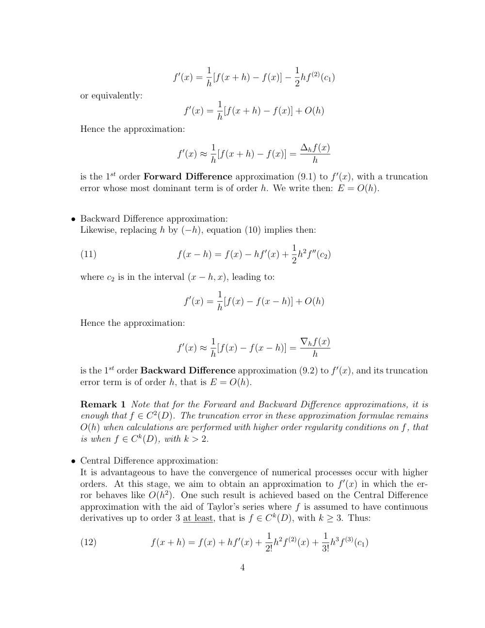• Forward Difference approximation: Using Taylor’s formula up to first order, we can write: f(x + h) = f(x) + hf ′(x) + 1 2h2f ′′(c1) (10) where c1 is in the interval (x, x + h), which leads to: 3 f ′(x) = 1 h[f(x + h) − f(x)] − 1 2hf (2)(c1) or equivalently: f ′(x) = 1 h[f(x + h) − f(x)] + O(h) Hence the approximation: f ′(x) ≈ 1 h[f(x + h) − f(x)] = ∆hf(x) h is the 1st order Forward Difference approximation (9.1) to f ′(x), with a truncation error whose most dominant term is of order h. We write then: E = O(h). • Backward Difference approximation: Likewise, replacing h by (−h), equation (10) implies then: f(x − h) = f(x) − hf ′(x) + 1 2h2f ′′(c2) (11) where c2 is in the interval (x − h, x), leading to: f ′(x) = 1 h[f(x) − f(x − h)] + O(h) Hence the approximation: f ′(x) ≈ 1 h[f(x) − f(x − h)] = ∇hf(x) h is the 1st order Backward Difference approximation (9.2) to f ′(x), and its truncation error term is of order h, that is E = O(h). Remark 1 Note that for the Forward and Backward Difference approximations, it is enough that f ∈ C2(D). The truncation error in these approximation formulae remains O(h) when calculations are performed with higher order regularity conditions on f, that is when f ∈ Ck(D), with k > 2. • Central Difference approximation: It is advantageous to have the convergence of numerical processes occur with higher orders. At this stage, we aim to obtain an approximation to f ′(x) in which the er- ror behaves like O(h2). One such result is achieved based on the Central Difference approximation with the aid of Taylor’s series where f is assumed to have continuous derivatives up to order 3 at least, that is f ∈ Ck(D), with k ≥ 3. 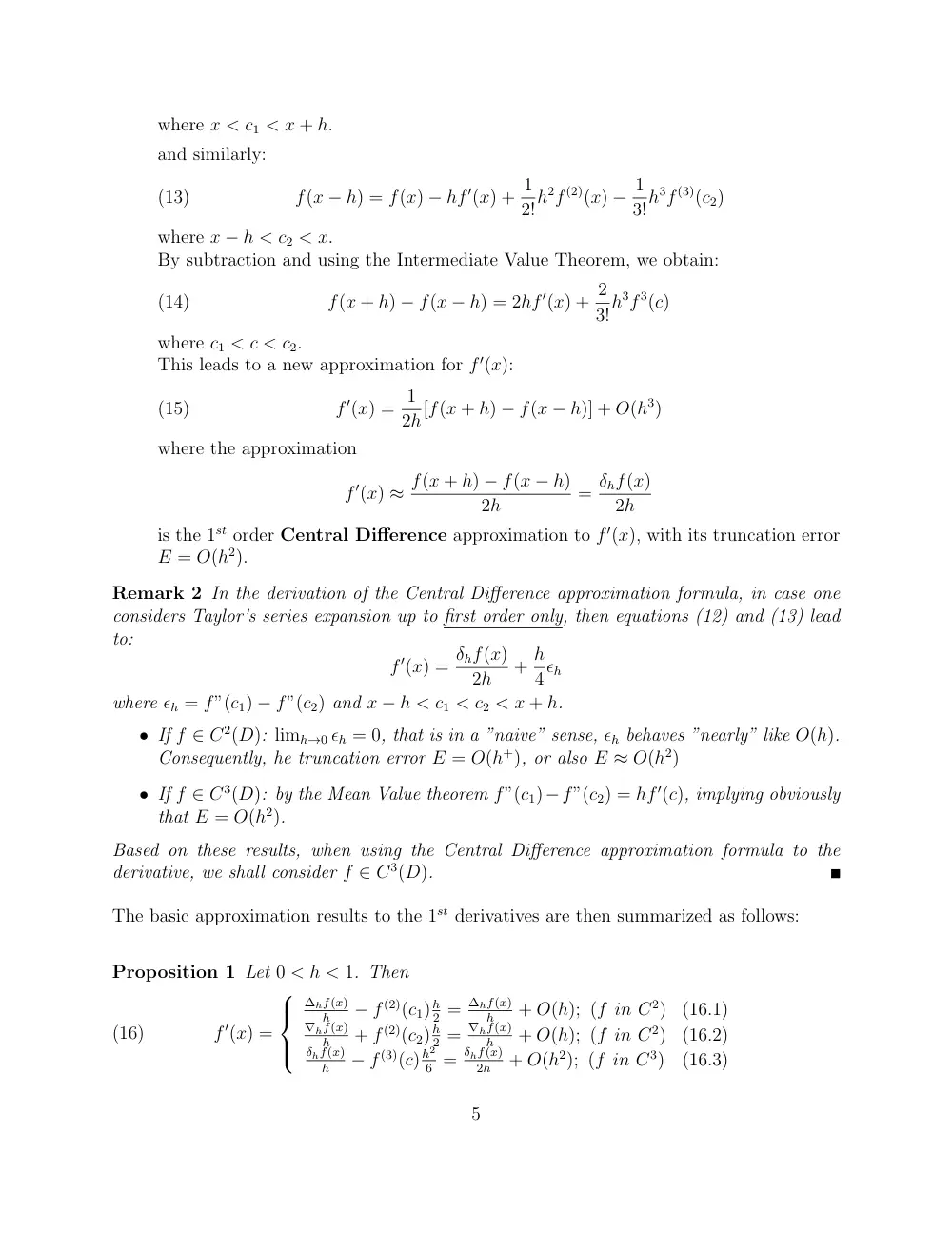Thus: f(x + h) = f(x) + hf ′(x) + 1 2!h2f (2)(x) + 1 3!h3f (3)(c1) (12) 4 where x < c1 < x + h. and similarly: f(x − h) = f(x) − hf ′(x) + 1 2!h2f (2)(x) − 1 3!h3f (3)(c2) (13) where x − h < c2 < x. By subtraction and using the Intermediate Value Theorem, we obtain: f(x + h) − f(x − h) = 2hf ′(x) + 2 3!h3f 3(c) (14) where c1 < c < c2. This leads to a new approximation for f ′(x): f ′(x) = 1 2h[f(x + h) − f(x − h)] + O(h3) (15) where the approximation f ′(x) ≈ f(x + h) − f(x − h) 2h = δhf(x) 2h is the 1st order Central Difference approximation to f ′(x), with its truncation error E = O(h2). Remark 2 In the derivation of the Central Difference approximation formula, in case one considers Taylor’s series expansion up to first order only, then equations (12) and (13) lead to: f ′(x) = δhf(x) 2h + h 4ϵh where ϵh = f”(c1) − f”(c2) and x − h < c1 < c2 < x + h. • If f ∈ C2(D): limh→0 ϵh = 0, that is in a ”naive” sense, ϵh behaves ”nearly” like O(h). Consequently, he truncation error E = O(h+), or also E ≈ O(h2) • If f ∈ C3(D): by the Mean Value theorem f”(c1)−f”(c2) = hf ′(c), implying obviously that E = O(h2). Based on these results, when using the Central Difference approximation formula to the derivative, we shall consider f ∈ C3(D). The basic approximation results to the 1st derivatives are then summarized as follows: Proposition 1 Let 0 < h < 1. 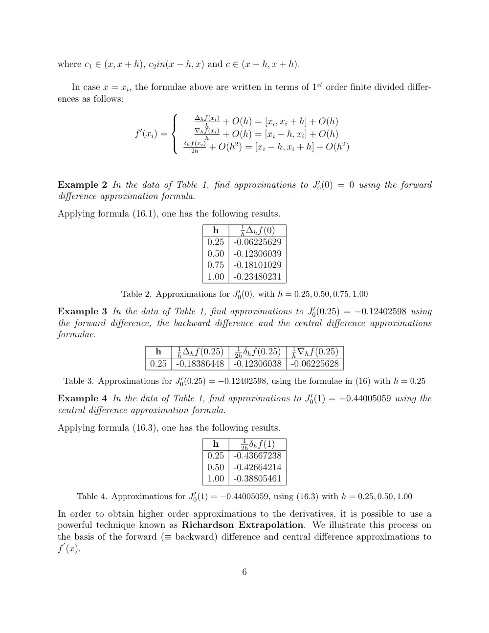Then f ′(x) =      ∆hf(x) h − f (2)(c1) h 2 = ∆hf(x) h + O(h); (f in C2) (16.1) ∇hf(x) h + f (2)(c2) h 2 = ∇hf(x) h + O(h); (f in C2) (16.2) δhf(x) h − f (3)(c) h2 6 = δhf(x) 2h + O(h2); (f in C3) (16.3) (16) 5 where c1 ∈ (x, x + h), c2in(x − h, x) and c ∈ (x − h, x + h). In case x = xi, the formulae above are written in terms of 1st order finite divided differ- ences as follows: f ′(xi) =      ∆hf(xi) h + O(h) = [xi, xi + h] + O(h) ∇hf(xi) h + O(h) = [xi − h, xi] + O(h) δhf(xi) 2h + O(h2) = [xi − h, xi + h] + O(h2) Example 2 In the data of Table 1, find approximations to J′ 0(0) = 0 using the forward difference approximation formula. Applying formula (16.1), one has the following results. h 1 h∆hf(0) 0.25 -0.06225629 0.50 -0.12306039 0.75 -0.18101029 1.00 -0.23480231 Table 2. Approximations for J′ 0(0), with h = 0.25, 0.50, 0.75, 1.00 Example 3 In the data of Table 1, find approximations to J′ 0(0.25) = −0.12402598 using the forward difference, the backward difference and the central difference approximations formulae. h 1 h∆hf(0.25) 1 2hδhf(0.25) 1 h∇hf(0.25) 0.25 -0.18386448 -0.12306038 -0.06225628 Table 3. Approximations for J′ 0(0.25) = −0.12402598, using the formulae in (16) with h = 0.25 Example 4 In the data of Table 1, find approximations to J′ 0(1) = −0.44005059 using the central difference approximation formula. Applying formula (16.3), one has the following results. h 1 2hδhf(1) 0.25 -0.43667238 0.50 -0.42664214 1.00 -0.38805461 Table 4. Approximations for J′ 0(1) = −0.44005059, using (16.3) with h = 0.25, 0.50, 1.00 In order to obtain higher order approximations to the derivatives, it is possible to use a powerful technique known as Richardson Extrapolation. We illustrate this process on the basis of the forward (≡ backward) difference and central difference approximations to f ′(x). 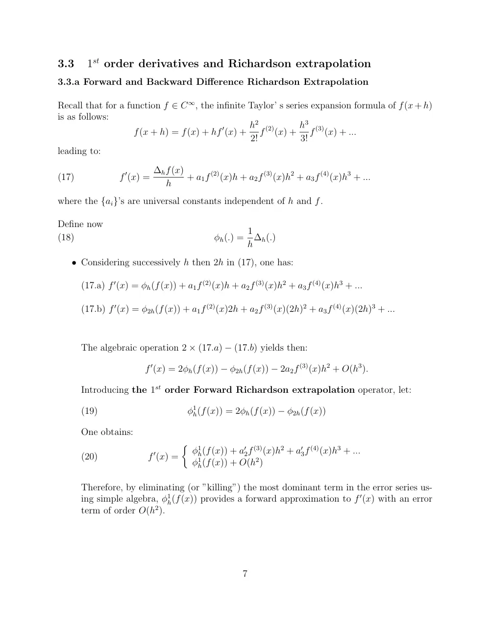6 3.3 1st order derivatives and Richardson extrapolation 3.3.a Forward and Backward Difference Richardson Extrapolation Recall that for a function f ∈ C∞, the infinite Taylor’ s series expansion formula of f(x + h) is as follows: f(x + h) = f(x) + hf ′(x) + h2 2! f (2)(x) + h3 3! f (3)(x) + ... leading to: f ′(x) = ∆hf(x) h + a1f (2)(x)h + a2f (3)(x)h2 + a3f (4)(x)h3 + ... (17) where the {ai}’s are universal constants independent of h and f. Define now φh(.) = 1 h∆h(.) (18) • Considering successively h then 2h in (17), one has: (17.a) f ′(x) = φh(f(x)) + a1f (2)(x)h + a2f (3)(x)h2 + a3f (4)(x)h3 + ... (17.b) f ′(x) = φ2h(f(x)) + a1f (2)(x)2h + a2f (3)(x)(2h)2 + a3f (4)(x)(2h)3 + ... The algebraic operation 2 × (17.a) − (17.b) yields then: f ′(x) = 2φh(f(x)) − φ2h(f(x)) − 2a2f (3)(x)h2 + O(h3). Introducing the 1st order Forward Richardson extrapolation operator, let: φ1 h(f(x)) = 2φh(f(x)) − φ2h(f(x)) (19) One obtains: f ′(x) = � φ1 h(f(x)) + a′ 2f (3)(x)h2 + a′ 3f (4)(x)h3 + ... φ1 h(f(x)) + O(h2) (20) Therefore, by eliminating (or ”killing”) the most dominant term in the error series us- ing simple algebra, φ1 h(f(x)) provides a forward approximation to f ′(x) with an error term of order O(h2). 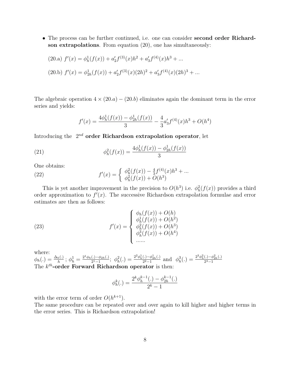7 • The process can be further continued, i.e. one can consider second order Richard- son extrapolations. From equation (20), one has simultaneously: (20.a) f ′(x) = φ1 h(f(x)) + a′ 2f (3)(x)h2 + a′ 3f (4)(x)h3 + ... (20.b) f ′(x) = φ1 2h(f(x)) + a′ 2f (3)(x)(2h)2 + a′ 3f (4)(x)(2h)3 + ... The algebraic operation 4 × (20.a) − (20.b) eliminates again the dominant term in the error series and yields: f ′(x) = 4φ1 h(f(x)) − φ1 2h(f(x)) 3 − 4 3a′ 3f (4)(x)h3 + O(h4) Introducing the 2nd order Richardson extrapolation operator, let φ2 h(f(x)) = 4φ1 h(f(x)) − φ1 2h(f(x)) 3 (21) One obtains: f ′(x) = � φ2 h(f(x)) − 4 3f (4)(x)h3 + ... φ2 h(f(x)) + O(h3) (22) This is yet another improvement in the precision to O(h3) i.e. φ2 h(f(x)) provides a third order approximation to f ′(x). The successive Richardson extrapolation formulae and error estimates are then as follows: f ′(x) =            φh(f(x)) + O(h) φ1 h(f(x)) + O(h2) φ2 h(f(x)) + O(h3) φ3 h(f(x)) + O(h4) ...... (23) where: φh(.) = ∆h(.) h ; φ1 h = 21φh(.)−φ2h(.) 21−1 ; φ2 h(.) = 22φ1 h(.)−φ1 2h(.) 22−1 and φ3 h(.) = 23φ2 h(.)−φ2 2h(.) 23−1 The kth-order Forward Richardson operator is then: φk h(.) = 2kφk−1 h (.) − φk−1 2h (.) 2k − 1 with the error term of order O(hk+1). The same procedure can be repeated over and over again to kill higher and higher terms in the error series. This is Richardson extrapolation! 8 Remark 3 In the process above, let φk h(.) = F(φk−1 h (.), φk−1 2h (.)) be the function approximat- ing the derivative f ′(.) in terms of 2 valid previous evaluations, with an error E = O(hk+1). Richardson extrapolation method allows to obtain an improved approximation formula φk h(.) without decreasing the value of h (that would favour increasing round-off errors). Thus through that process, the new approximation is ”extrapolated” to the exact value of the deriva- tive. 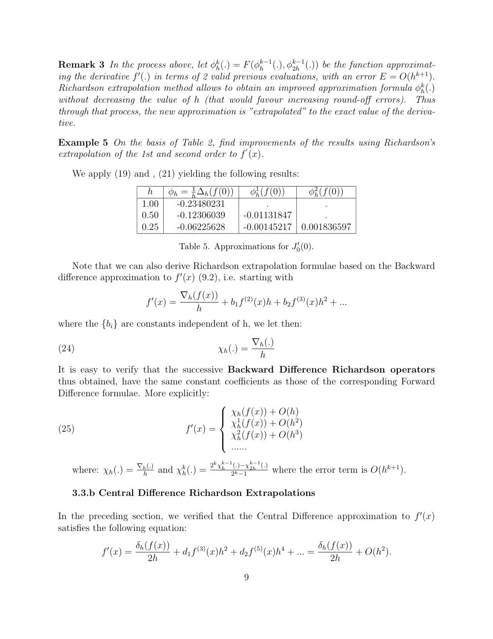Example 5 On the basis of Table 2, find improvements of the results using Richardson’s extrapolation of the 1st and second order to f ′(x). We apply (19) and , (21) yielding the following results: h φh = 1 h∆h(f(0)) φ1 h(f(0)) φ2 h(f(0)) 1.00 -0.23480231 . . 0.50 -0.12306039 -0.01131847 . 0.25 -0.06225628 -0.00145217 0.001836597 Table 5. Approximations for J′ 0(0). Note that we can also derive Richardson extrapolation formulae based on the Backward difference approximation to f ′(x) (9.2), i.e. starting with f ′(x) = ∇h(f(x)) h + b1f (2)(x)h + b2f (3)(x)h2 + ... where the {bi} are constants independent of h, we let then: χh(.) = ∇h(.) h (24) It is easy to verify that the successive Backward Difference Richardson operators thus obtained, have the same constant coefficients as those of the corresponding Forward Difference formulae. More explicitly: f ′(x) =        χh(f(x)) + O(h) χ1 h(f(x)) + O(h2) χ2 h(f(x)) + O(h3) ...... (25) where: χh(.) = ∇h(.) h and χk h(.) = 2kχk−1 h (.)−χk−1 2h (.) 2k−1 where the error term is O(hk+1). 3.3.b Central Difference Richardson Extrapolations In the preceding section, we verified that the Central Difference approximation to f ′(x) satisfies the following equation: f ′(x) = δh(f(x)) 2h + d1f (3)(x)h2 + d2f (5)(x)h4 + ... = δh(f(x)) 2h + O(h2). 9 With such information, it is possible to rely again on the powerful technique of Richardson extrapolation to wring more accuracy out of the method in the approximation-formulae of f ′(x). Specifically, let ψh(.) = δh(.) 2h Obviously, then: f ′(x) = ψh(f(x)) + d1f (3)(x)h2 + d2f (5)(x)h4 + ... = ψh(f(x)) + O(h2) (26) Taking successively h then 2h in the equation above, one has: (26.a) f ′(x) = ψh(f(x)) + d1f (3)(x)h2 + d2f (5)(x)h4 + ... (26.b) f ′(x) = ψ2h(f(x)) + d1f (3)(x)(2h)2 + d2f (5)(x)(2h)4 + ... The algebraic operation 4 × (26.a) − (26.b) yields: f ′(x) = 4ψh(f(x)) − ψ2h(f(x)) 3 + O(h4) Let the 1st order Richardson extrapolation operator be defined by ψ1 h(.) = 22ψh(.) − ψ2h(.) 22 − 1 One can write then: f ′(x) = ψ1 h(f(x)) + O(h4) (27) Leading therefore to the following identities: (27.a) f ′(x) = ψ1 h(f(x)) + d′ 2f (5)(x)h4 + d′ 3f (7)(x)h6 + ... (27.b) f ′(x) = ψ1 2h(f(x)) + d′ 2f (5)(x)(2h)4 + d′ 3f (7)(x)(2h)6 + ... The algebraic operation 16 × (27.a) − (27.b) yields: f ′(x) = 24ψ1 h(f(x)) − ψ1 2h(f(x)) 24 − 1 + O(h6) or equivalently: f ′(x) = ψ2 h(f(x)) + O(h6) Again, the process can be repeated to obtain higher order accuracy in the approximations of f ′(x). 10 Therefore, the 1st Central Difference Richardson extrapolation formulae obtained are as follows: f ′(x) =        ψh(f(x)) + O(h2) ψ1 h(f(x)) + O(h4) ψ2 h(f(x)) + O(h6) ...... (28) where ψh(.) = δh(.) 2h , ψ1 h(.) = 22ψh(.)−ψ2h(.) 22−1 , ψ2 h(.) = 24ψ1 h(.)−ψ1 2h(.) 24−1 .... The kth-order operator is then defined as follows: ψk h(.) = 22kψk−1 h (.) − ψk−1 2h (.) 22k − 1 where the error term is O(h2k+2) 3.4 2nd Order Derivatives and Divided Differences.Error Analysis A direct application of Theorem 1 with k = 2 suggests the following approximation formulae for the 2nd derivative of f: f ′′(xi) ≈      2[xi, xi+1, xi+2] = yi+2−2yi+1+yi h2 = ∆2 hyi h2 ; Forward Difference 2[xi−2, xi−1, xi] = yi−2yi−1+yi−2 h2 = ∇2 hyi h2 ; Backward Difference 2[xi−1, xi, xi+1] = yi+1−2yi+yi−1 h2 = δ2 hyi h2 ; Central Difference We start by estimating the order of convergence of each approximation formula: • Forward Difference approximation Consider the 2 Taylor’s series expansions of f up to 2nd order given by: (i) f(x + h) = f(x) + h 1!f ′(x) + h2 2! f ′′(x) + h3 3! f (3)(c1) ; c1 ∈ (x, x + h) (ii) f(x + 2h) = f(x) + (2h) 1! f ′(x) + (2h)2 2! f ′′(x) + (2h)3 3! f (3)(c2) ; c2 ∈ (x, x + 2h) where f is assumed to be a C3-function. The algebraic operation: f(x + 2h) − 2f(x + h) leads to the Forward Difference Approximation to f ′′(x) verifying the following: f ′′(x) = f(x + 2h) − 2f(x + h) + f(x) h2 + O(h) = ∆2 hf(x) h2 + O(h) (29) • Backward Difference approximation Furthermore, replacing h by −h in equations (i) and (ii) above, one also has: (iii) f(x − h) = f(x) − h 1!f ′(x) + h2 2! f ′′(x) − h3 3! f (3)(c3) ; c3 ∈ (x − h, x) 11 (iv) f(x − 2h) = f(x) − (2h) 1! f ′(x) + (2h)2 2! f ′′(x) − (2h)3 3! f (3)(c4) ; c4 ∈ (x − 2h, x+) The algebraic operation: f(x − 2h) − 2f(x − h) leads to the Backward Difference Approximation to f ′′(x) verifying the following: f ′′(x) = f(x − 2h) − 2f(x − h) + f(x) h2 + O(h) = ∇2 hf(x) h2 + O(h) (30) • Central Difference approximation In this case we start by writing Taylor’s series expansions up to the 3rd order succes- sively for f(x + h and f(x − h) and then sum up the two series. This leads to: f(x + h) + f(x − h) = 2f(x) + f ′′(x)h2 + h4 4! (f (4)(c1) + f (4)(c2)) Dividing by h2 and using the Intermediate Value Theorem, one concludes that: f ′′(x) = f(x + h) − 2f(x) + f(x − h) h2 − h2 12f (4)(c) = δ2 h h2(f(x)) + O(h2) Based on the results above, the following proposition is satisfied: Proposition 2 Let 0 < h ≤ 1. Then f ′′(x) =      ∆2 hf(x) h2 + O(h), (31.1) ∇2 hf(x) h2 + O(h), (31.2) δ2 hf(x) h2 + O(h2), (31.3) (31) where f is assumed to have up to third order continuous derivatives for the first 2 approxi- mations (f ∈ C3), and up to fourth order continuous derivatives for the third approximation (f ∈ C4). In terms of finite differences, these results are expressed as follows: f ′′(xi) ≈      2[xi, xi+1, xi+2] = ∆2 hyi h2 + O(h); Forward Difference 2[xi−2, xi−1, xi] = ∇2 hyi h2 + O(h); Backward Difference 2[xi−1, xi, xi+1] = δ2 hyi h2 + O(h2); Central Difference Remark 4 Based on Theorem 1, the following approximation formulae for the 3rd derivative of f are obtained: f ′′′(xi) ≈      6[xi, xi+1, xi+2, xi+3] = ∆3 hyi h3 ; ForwardDifference 6[xi−3, xi−2, xi−1, xi] = ∇3 hyi h3 ; BackwardDifference 6[xi−2, xi−1, xi+1, xi+2] = δ3 hyi h3 ; CentralDifference 12 3.5 2nd order derivatives and Richardson Extrapolation In order to improve the order of the approximations of the 2nd derivative, we can use as pre- cedingly the powerful tool of Richardson extrapolation applied successively to the Forward, Backward and Central Difference formulae. In this section, we analyze only the Richardson extrapolation Central Difference ap- proximation to f ′′(x). In the equations above: f ′′(x) ≈ f(x + h) − 2f(x) + f(x − h) h2 = δ2 hf(x) h2 (32) Define then: ψh(.) = δ2 h(.) h2 Adding the infinite series for f(x + h) and f(x − h), one can write successively: f ′′(x) = ψh(f(x)) + d1f (4)(x)h2 + d2f (6)(x)h4 + ... (33) f ′′(x) = ψ2h(f(x)) + d1f (4)(x)(2h)2 + d2f (6)(x)(2h)4 + ... (34) In order to eliminate the most dominant term of the error in the above 2 series, the algebraic operation 4 × (33) − (34) yields: f ′′(x) = 4ψh(f(x)) − ψ2h(f(x)) 3 + O(h4) (35) Defining the 1st order Richardson extrapolation operator by ψ1 h(.) = 22ψh(.) − ψ2h(.) 22 − 1 , one rewrites (35) as: f ′′(x) = ψ1 h(f(x)) + O(h4) which improves the order of approximation. Obviously, one can derive the following estimates: f ′′(x) =        ψh(f(x)) + O(h2) ψ1 h(f(x)) + O(h4) ψ2 h(f(x)) + O(h6) ...... (36) where ψh(.) = δ2 h(.) 2h , ψ1 h(.) = 22ψh(.)−ψ2h(.) 22−1 , ψ2 h(.) = 24ψ1 h(.)−ψ1 2h(.) 24−1 . 13 4 Numerical Integration We consider now the approximation of I(a, b) ≡ � b a f(x)dx, based on the data Dn. As in the numerical differentiation process, we assume the x-data to be equidistant, with: h = xi+1 − xi, ∀i. Depending on the parity of n (i.e on the number of subintervals), we start by decomposing the integral I into the sum of simple integrals over the subintervals [xi, xi+1] as follows: I = � x1 x0 f(x)dx + � x2 x1 f(x)dx + ... + � xn xn−1 f(x)dx = n−1 � k=0 � xk+1 xk f(x)dx, ∀n and in particular: I = � x2 x0 f(x)dx + � x4 x2 f(x)dx + ... + � x2m x2m−2 f(x)dx = m−1 � k=0 � x2k+2 x2k f(x)dx, ∀n = 2m Thus, we will be dealing with 2 types of formulae: 1. Simple Numerical integration formulae Ik = � xk+1 xk f(x)dx ∀ n , or I′ k = � x2k+2 x2k f(x)dx , ∀ n = 2m Subsequently, 2. Composite Numerical integration formulae I = � b a f(x)dx = n−1 � k=0 Ik ∀ n , or I = � b a f(x)dx = m−1 � k=0 I′ k , ∀ n = 2m We start with the simplest approximation method, called the Midpoint Rectangular Rule. 4.1 The Midpoint Rectangular Rule Such rule applies only in the case when the number of subintervals is even, that is when n = 2m. 1. The formulae A simple geometric argument consists in considering the integral I′ k as being the area of the region between the x- axis, the curve y = f(x) and the vertical lines x = x2k and x = x2k+2. Such area is then approximated by the surface of the rectangle which vertical sides are x = x2k and x = x2k+2, and horizontal sides y = 0 and y = f(x2k+1). In such case, the function values at the midpoints are known. For example, in the case of the data in Table 1, 14 i xi f(xi) 0 0.00 1.0000000 1 0.25 0.98443593 2 0.50 0.93846981 3 0.75 0.86424228 4 1.00 0.76519769 5 1.25 0.64590609 6 1.50 0.51182767 7 1.75 0.36903253 8 2.00 0.22389078 the set of midpoints is {x1, x3, x5, x7}.This leads first to the simple Midpoint (rect- angular) rule, given by: I′ k = � x2k+2 x2k f(x)dx ≈ Mk = 2hf(x2k+1), k = 0, 1, ..., m − 1. (37) and subsequently to the composite Midpoint rule given by: I ≡ I(a, b) = � b a f(x)dx ≈ M(h) = Σm−1 k=0 2hf(x2k+1) (38) 2. Error analysis The error analysis of this method is based on either one of Taylor’s formulae where the expansion is made about the point x = x2k+1, yielding: f(x) = f(x2k+1) + f ′(x2k+1)(x − x2k+1) + f ′′(ck(x))(x − x2k+1)2 2 (39) where ck(x) = x2k+1 + t(x − x2k+1), 0 < t < 1. Obviously, it is required that the function f is at least in C2[a, b]. Integration of equation (39) from x2k to x2k+2 and the use of the second Mean-value theorem leads to: � x2k+2 x2k f(x)dx = 2hf(x2k+1) + f ′′(ck) � x2k+2 x2k (x − x2k+1)2 2 dx (40) where ck is a point in (x2k, x2k+2). One easily verifies that the integrals of odd powers of (x − x2k+1) in (39) cancel out, with only the integrals of even powers contributing to the final result, thus yielding: I′ k = Mk + f ′′(ck)h3 3 (41) 15 Summing up (41) over k yields: I(a, b) = m−1 � k=0 I′ k = m−1 � k=0 Mk + h3 3 m−1 � k=0 f ′′(ck) = M(h) + h3 3 m−1 � k=0 f ′′(ck). Using the intermediate value theorem, one has: m−1 � k=0 f ′′(ck) = mf ′′(d) = b − a 2h f”(d), d ∈ (a, b) and therefore, noting that the length of the interval of integration is nh = (2m)h = b − a the following result is reached: I = I(a, b) = M(h) + (b − a) 6 f ′′(d)h2 (42) Proposition 3 Let f be a function in C2[a, b], interpolating the set of data Dn where n = 2m. Then I = � b a f(x)dx = M(h) + O(h2) where M(h) = 2h m−1 � k=0 f(x2k+1) Furthermore, when h = b−a 2l , l = 0, 1, 2, ..., it can be proved that: I = I(a, b) = M(h) + µ1h2 + µ2h4 + .. + µjh2j + ..., (43) where the sequence {µj} is independent from h, and depends on the function f (and its derivatives) at a and b. 4.2 The Trapezoidal Rule Unlike the composite Midpoint rule that is only applicable when the number of intervals is even, the composite Trapezoid rule can be used in all cases. 1. The formulae A simple geometric argument consists in approximating the surface between the x-axis, the curve y = f(x) and the vertical lines x = xk and x = xk+1 by the area of the rect- angular trapezoid, which vertices are (xk, 0), (xk+1, 0), (xk, f(xk)) and (xk+1, f(xk+1)). This leads first to the simple Trapezoidal rule, given by: Ik = � xk+1 xk f(x)dx ≈ Tk = h 2(f(xk) + f(xk+1)), (44) 16 and subsequently to the composite Trapezoid rule given by: I ≡ I(a, b) = � b a f(x)dx ≈ T(h) = h 2 Σn−1 k=0(f(xk) + f(xk+1)), (45) More precisely: T(h) = h 2 (y0 + 2(y1 + ... + yn−1) + yn) Remark 5 Note that when n = 2m, then: I ≈ T(2h) = Σm−1 k=0 T ′ k = Σm−1 k=0 h(f(x2k + f(x2k+2)) On the other hand: M(h) = Σm−1 k=0 Mk = 2hΣm−1 k=0 f(x2k+1) Considering then (T(2h) + M(h))/2, one gets: T(h) = 1 2(T(2h) + M(h)) (46) To prove this result note that: T(2h) + M(h) = h m−1 � k=0 (f(x2k) + f(x2k+2)) + 2f(x2k+1) = = h m−1 � k=0 [f(x2k) + f(x2k+1)] + [f(x2k+1) + f(x2k+2)] = h n−1 � k=0 (f(xk) + f(xk+1)) = 2T(h). This result is summarized in: Proposition 4 For n = 2m, T(h) = 1 2(T(2h) + M(h)). 2. Error analysis Note that: Tk = � xk+1 xk pk,k+1(x)dx (47) where pk,k+1(x) = yk +[xk, xk+1](x−xk), is the linear interpolation polynomial to f(x) at xk and xk+1. Furthermore, it is well known (section 4.5) that: f(x) = pk,k+1(x) + 1 2(x − xk)(x − xk+1)f ′′(c(x)), 17 with c(x) ∈ (xk, xk+1) depending continuously on x. By integration of this identity over the interval (xk, xk+1) and use of the second Mean Value Theorem with (47), one gets: Ik = Tk + f ′′(ck) 2 � xk+1 xk (x − xk)(x − xk+1) dx leading to: Ik = Tk − h3 12f ′′(ck), (48) where ck ∈ (xk, xk+1). Summing up (48) over k, one gets an expression for the com- posite Trapezoidal rule error term (likewise for the Midpoint rule in (42)): I = I(a, b) = n−1 � k=0 Ik = T(h) − (b − a) 12 f ′′(c)h2 (49) where c ∈ (a, b). Proposition 5 Let the data Dn = {(xk, f(xk))|k = 0, 1, ..., n}, be a set representing a function f in C2([a, b]), then: I = � b a f(x)dx = T(h) + O(h2), with: T(h) = h 2Σn−1 k=0(f(xk) + f(xk+1)). On the other hand, as in (43), can prove that when h = b−a 2l , l = 0, 1, 2, ...: I = I(a, b) = T(h) + τ1h2 + τ2h4 + .. + τjh2j + ..., (50) where the sequence {τj} depends on the function f (and its derivatives) at a and b and consequently independent from h. 4.3 Trapezoid Rule / Richardson’s extrapolation: Romberg for- mulae 1. The formulae On the basis of (50), we can implement Richardson’s extrapolation, by writing this equation simultaneously for h and h 2. Specifically, in that case we obtain: (a) I = T(h) + τ1h2 + τ2h4 + ... + τjh2j + ... (b) I = T � h 2 � + τ1 � h 2 �2 + τ2 � h 2 �4 + ... + τj � h 2 �2j + ... 18 In order to eliminate the dominant term of the error, by performing the algebraic operation 4(b) − (a), we obtain: 3I = 4T �h 2 � − T(h) + O(h4) and therefore: I = 4T � h 2 � − T(h) 3 + t2h4 + t3h6 + ... (51) where the sequence {ti} is independent of h. Defining the first Romberg integration operator as: R1(h/2) = 4T � h 2 � − T(h) 3 or equivalently R1(h) = 4T(h) − T(2h) 3 (52) equation (51) provides then an approximation to the integral I(a, b) of order O(h4) verifying: I = R1(h) + O(h4) (53) In a similar way, we can derive a second Romberg integration formula by writing again the equation above simultaneously in terms of h and h 2: (a) I = R1(h) + t2h4 + t3h6 + ... (b) I = R1 � h 2 � + t2 � h 2 �4 + t3 � h 2 �6 + ... Performing the algebraic operation 16(b) − (a) yields: 15I = 16R1 �h 2 � − R1(h) + O(h6) And therefore: I = 16R1 � h 2 � − R1(h) 15 + t3h6 + t4h8 + ... (54) where the sequence {ti} is independent of h. Defining the second Romberg integration operator as: R2(h) = 16R1(h) − R1(2h) 15 (55) equation (5.52) is then equivalent to: I = R2(h) + O(h6) (56) As for differentiation, this process can be repeated. The first Romberg extrapolation formulae obtained based on the Composite Trapezoid Rule are as follows: 19 Proposition 6 Let f belong to C∞[a, b] I = I(a, b) = � b a f(x)dx =        R1(h) + O(h4) R2(h) + O(h6) R3(h) + O(h8) ... Where R1(h) = 22T(h)−T(2h) 22−1 ; R2(h) = 24R1(h)−R1(2h) 24−1 ; R3(h) = 26R2(h)−R2(2h) 26−1 , and in general: Rk(h) = 22kRk−1(h)−Rk−1(2h) 22k−1 , 2. Simpson’s Rule Simpson’s Rule is applicable only if the number of subintervals is even (n=2m). It can be derived from a linear combination of the Midpoint Rule and the Trapezoid Rule. Specifically, the simple integration Simpson’s Rule is defined as follows Sk = 2 3Mk + 1 3Tk (57) Consequently: Sk = 2 3[f(x2k+1)2h] + 1 3[f(x2k) + f(x2k+1) 2 2h] leading to: I′ k = � x2k+2 x2k f(x)dx ≈ Sk = h 3(f(x2k) + 4f(x2k+1) + f(x2k+2)) (58) Summing up this last equation over k, one derives the Composite Simpson’s Rule, namely: I = I(a, b) = Σm−1 k=0 Sk = Σm−1 k=0 (2 3Mk + 1 3Tk) = 2M(h) + T(2h) 3 (59) Referring to Proposition (4), since M(h) = 2T(h) − T(2h), then one concludes that: S(h) = 4T(h) − T(2h) 3 = R1(h) meaning that Simpson’s Composite Numerical Integration formula is equivalent to the first Romberg Trapezoidal Extrapolation formula. Thus, the following error estimate is obviously deduced: Proposition 7 Let f be a function in C4[a, b], interpolating the set of data Dn. Then: I = I(a, b) = S(h) + O(h4) 20 Remark 6 The error estimate of the Composite Simpson’s rule can also be derived by noting that Sk = � x2k+2 x2k p2k,2k+1,2k+2(x)dx where p2k,2k+1,2k+2(x) is the quadratic interpolating polynomial to f(x) at x2k, x2k+1, x2k+2. Specifically one proves that: Ik = Sk − 1 90f (4)(ck(x))h5. leading therefore to: I = S(h) − (b − a) 1 180f (4)(c)h4. where S(h) = (y0 + 4 �m−1 k=0 y2k+1 + 2(�m−1 k=1 y2k) + y2m) h 3 In a consistent manner with the Composite Midpoint and Trapezoidal Rules, one also has when h = b−a 2l , l = 0, 1, 2, ...: I = I(a, b) = S(h) + s2h4 + s6h6 + .... + sjh2j + .... where all the coefficients {si} are independent of h. In the last part of this chapter, we explore a totally different approach of estimating definite integrals. We will show that we can use sequences of random numbers for these approximations, a problem that seemingly has nothing to do with randomness. 5 Monte Carlo Methods and Random Numbers 21 PROBLEMS Numerical Differentiation 1. If φ(h) = L−c1h−c2h2 −c3h3 −..., then what combination of φ(h) and φ(h/2) should give an accurate estimate of L ? 2. If φ(h) = L − c1h1/2 − c2h2/2 − c3h3/2 − ..., then what combination of φ(h) and φ(h/2) should give an accurate estimate of L ? 3. Consider the following table of data associated with some unknown function y = f(x) i xi yi 0 0.0