
MATH 251 Notes Chapter 4, Spring 2014
American University of Beirut · Numerical Computing · 46 pages


Showing the first 10 of 46 pages. Download the PDF to see all of it.
More MATH 251 files
Show the text of this notes
Chapter 4
Polynomial Interpolation and
Splines Fitting
4.1
Definition of Interpolation
Consider a set Dn of n + 1 data points in the (x, y) plane:
(4.1)
Dn = {(xi, yi)| i = 0, 1 ..., n; n 2 N with xi 6= xj for i 6= j}.
We assume that Dn represents partially the values of a function y = f(x),
i.e.:
(4.2)
f(xi) = yi 8 i = 0, 1 ..., n
Our basic objective in this chapter is to construct a continuous function r(x)
that “represents” f(x) (or the empirical law f(x) behind the set of data Dn).
Thus r(x) would represent f(x) for all x, in particular for x 62 the set of
nodes {x0, x1, ..., xn}. Such a function r(x) is said to interpolate the set
of data Dn if it satisfies the interpolation conditions:
(4.3)
r(xi) = yi 8 i = 0, 1 ..., n
i.e. fitting the function f(x) at the nodes {xi}, .
Several kinds of interpolation may be considered by choosing r(x) to be a
polynomial function, a rational function or even a trigonometric one. The
most natural is to consider polynomial or piecewise polynomial interpolation
(spline functions) , as polynomial functions are the simplest in reproduc-
ing the basic arithmetic (floating-point) operations of addition, subtraction,
143
144
N. Nassif and D. Fayyad
multiplication and division {+, −, ⇥, ÷}. Consistently, we only analyze in
this chapter polynomial and spline interpolations. Such type of inter-
polation is referred to as Lagrange interpolation.
4.2
General Lagrange Polynomial Interpolation
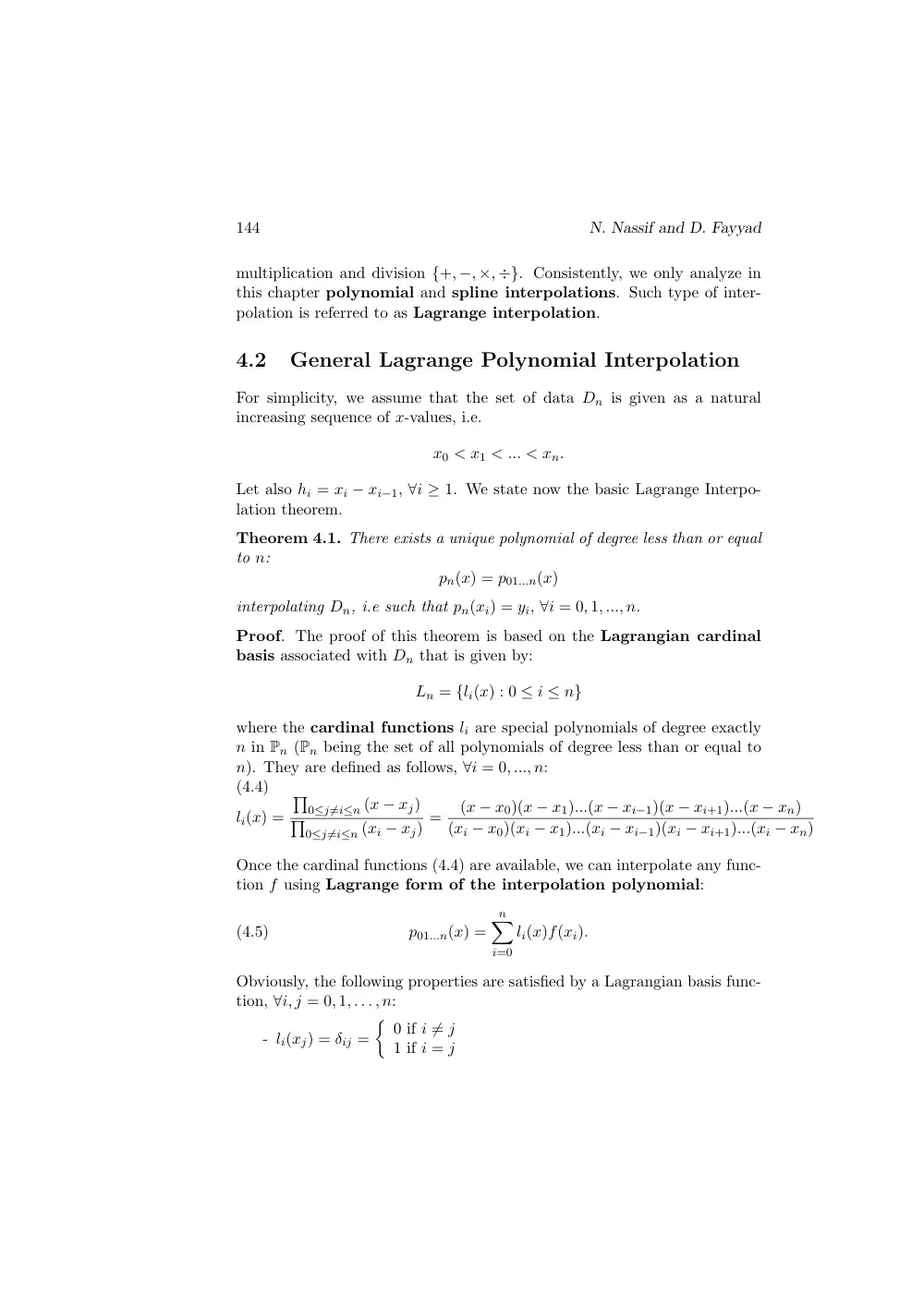
For simplicity, we assume that the set of data Dn is given as a natural
increasing sequence of x-values, i.e.
x0 < x1 < ... < xn.
Let also hi = xi − xi−1, 8i ≥ 1. We state now the basic Lagrange Interpo-
lation theorem.
Theorem 4.1. There exists a unique polynomial of degree less than or equal
to n:
pn(x) = p01...n(x)
interpolating Dn, i.e such that pn(xi) = yi, 8i = 0, 1, ..., n.
Proof. The proof of this theorem is based on the Lagrangian cardinal
basis associated with Dn that is given by:
Ln = {li(x) : 0 i n}
where the cardinal functions li are special polynomials of degree exactly
n in Pn (Pn being the set of all polynomials of degree less than or equal to
n). They are defined as follows, 8i = 0, ..., n:
(4.4)
li(x) =
Q
0j6=in (x − xj)
Q
0j6=in (xi − xj) =
(x − x0)(x − x1)...(x − xi−1)(x − xi+1)...(x − xn)
(xi − x0)(xi − x1)...(xi − xi−1)(xi − xi+1)...(xi − xn)
Once the cardinal functions (4.4) are available, we can interpolate any func-
tion f using Lagrange form of the interpolation polynomial:
(4.5)
p01...n(x) =
n
X
i=0
li(x)f(xi).
Obviously, the following properties are satisfied by a Lagrangian basis func-
tion, 8i, j = 0, 1, . . . , n:
- li(xj) = δij =
⇢ 0 if i 6= j
1 if i = j
Polynomial and Splines Interpolation
145
- p01...n(xi) = yi
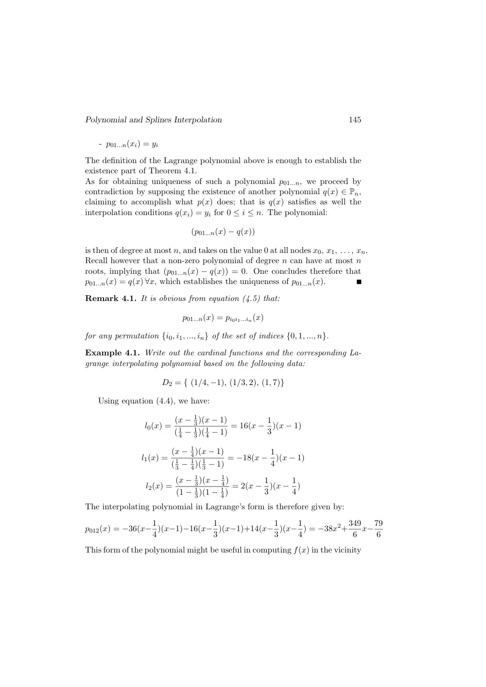
The definition of the Lagrange polynomial above is enough to establish the
existence part of Theorem 4.1.
As for obtaining uniqueness of such a polynomial p01...n, we proceed by
contradiction by supposing the existence of another polynomial q(x) 2 Pn,
claiming to accomplish what p(x) does; that is q(x) satisfies as well the
interpolation conditions q(xi) = yi for 0 i n. The polynomial:
(p01...n(x) − q(x))
is then of degree at most n, and takes on the value 0 at all nodes x0, x1, . . . , xn.
Recall however that a non-zero polynomial of degree n can have at most n
roots, implying that (p01...n(x) − q(x)) = 0. One concludes therefore that
p01...n(x) = q(x) 8x, which establishes the uniqueness of p01...n(x).
Remark 4.1. It is obvious from equation (4.5) that:
p01...n(x) = pi0i1...in(x)
for any permutation {i0, i1, ..., in} of the set of indices {0, 1, ..., n}.
Example 4.1. Write out the cardinal functions and the corresponding La-
grange interpolating polynomial based on the following data:
D2 = { (1/4, −1), (1/3, 2), (1, 7)}
Using equation (4.4), we have:
l0(x) = (x − 1
3)(x − 1)
( 1
4 − 1
3)( 1
4 − 1) = 16(x − 1
3)(x − 1)
l1(x) = (x − 1
4)(x − 1)
( 1
3 − 1
4)( 1
3 − 1) = −18(x − 1
4)(x − 1)
l2(x) = (x − 1
3)(x − 1
4)
(1 − 1
3)(1 − 1
4) = 2(x − 1
3)(x − 1
4)
The interpolating polynomial in Lagrange’s form is therefore given by:
p012(x) = −36(x−1
4)(x−1)−16(x−1
3)(x−1)+14(x−1
3)(x−1
4) = −38x2+349
6 x−79
6
This form of the polynomial might be useful in computing f(x) in the vicinity
146
N. Nassif and D. Fayyad
of the nodes 1/3, 1/4, 1.
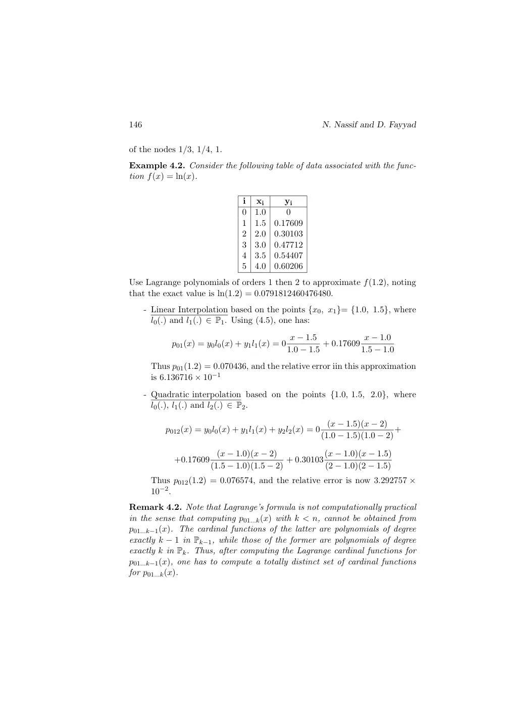
Example 4.2. Consider the following table of data associated with the func-
tion f(x) = ln(x).
i
xi
yi
0
1.0
0
1
1.5
0.17609
2
2.0
0.30103
3
3.0
0.47712
4
3.5
0.54407
5
4.0
0.60206
Use Lagrange polynomials of orders 1 then 2 to approximate f(1.2), noting
that the exact value is ln(1.2) = 0.0791812460476480.
- Linear Interpolation based on the points {x0, x1}= {1.0, 1.5}, where
l0(.) and l1(.) 2 P1. Using (4.5), one has:
p01(x) = y0l0(x) + y1l1(x) = 0 x − 1.5
1.0 − 1.5 + 0.17609 x − 1.0
1.5 − 1.0
Thus p01(1.2) = 0.070436, and the relative error iin this approximation
is 6.136716 ⇥ 10−1
- Quadratic interpolation based on the points {1.0, 1.5, 2.0}, where
l0(.), l1(.) and l2(.) 2 P2.
p012(x) = y0l0(x) + y1l1(x) + y2l2(x) = 0
(x − 1.5)(x − 2)
(1.0 − 1.5)(1.0 − 2)+
+0.17609
(x − 1.0)(x − 2)
(1.5 − 1.0)(1.5 − 2) + 0.30103(x − 1.0)(x − 1.5)
(2 − 1.0)(2 − 1.5)
Thus p012(1.2) = 0.076574, and the relative error is now 3.292757 ⇥
10−2.
Remark 4.2. Note that Lagrange’s formula is not computationally practical
in the sense that computing p01...k(x) with k < n, cannot be obtained from
p01...k−1(x). The cardinal functions of the latter are polynomials of degree
exactly k − 1 in Pk−1, while those of the former are polynomials of degree
exactly k in Pk. Thus, after computing the Lagrange cardinal functions for
p01...k−1(x), one has to compute a totally distinct set of cardinal functions
for p01...k(x).
Polynomial and Splines Interpolation
147
This motivates looking for recurrence formulae to the Lagrange interpolating
polynomial.
4.3
Recurrence Formulae
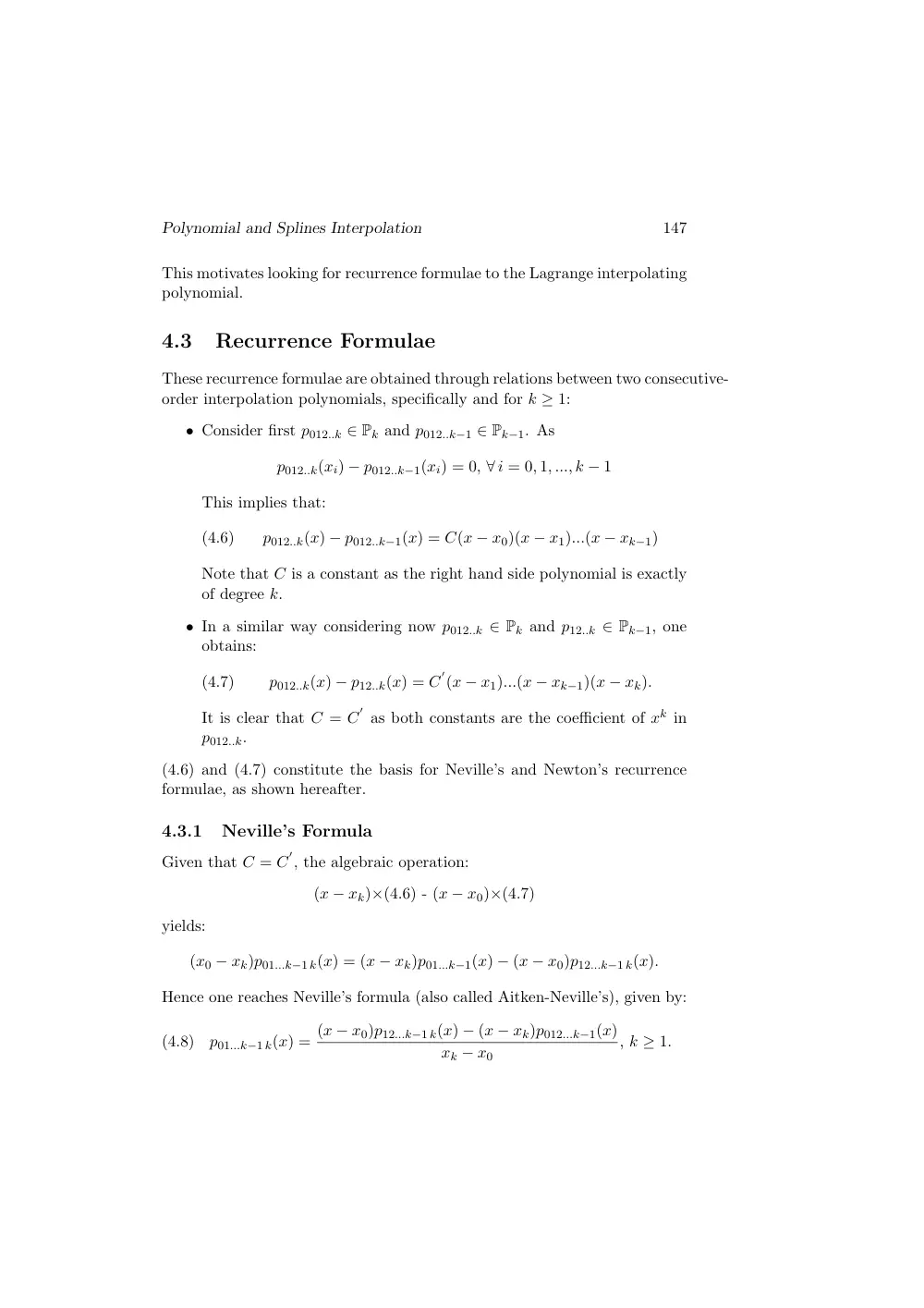
These recurrence formulae are obtained through relations between two consecutive-
order interpolation polynomials, specifically and for k ≥ 1:
• Consider first p012..k 2 Pk and p012..k−1 2 Pk−1. As
p012..k(xi) − p012..k−1(xi) = 0, 8 i = 0, 1, ..., k − 1
This implies that:
(4.6)
p012..k(x) − p012..k−1(x) = C(x − x0)(x − x1)...(x − xk−1)
Note that C is a constant as the right hand side polynomial is exactly
of degree k.
• In a similar way considering now p012..k 2 Pk and p12..k 2 Pk−1, one
obtains:
(4.7)
p012..k(x) − p12..k(x) = C
0(x − x1)...(x − xk−1)(x − xk).
It is clear that C = C
0 as both constants are the coefficient of xk in
p012..k.
(4.6) and (4.7) constitute the basis for Neville’s and Newton’s recurrence
formulae, as shown hereafter.
4.3.1
Neville’s Formula
Given that C = C
0, the algebraic operation:
(x − xk)⇥(4.6) - (x − x0)⇥(4.7)
yields:
(x0 − xk)p01...k−1 k(x) = (x − xk)p01...k−1(x) − (x − x0)p12...k−1 k(x).
Hence one reaches Neville’s formula (also called Aitken-Neville’s), given by:
(4.8)
p01...k−1 k(x) = (x − x0)p12...k−1 k(x) − (x − xk)p012...k−1(x)
xk − x0
, k ≥ 1.
148
N. Nassif and D. Fayyad
A more general Neville’s recurrence formulae can be concluded. Specif-
ically, for any i 2 {0, 1, ..., n}. :
• Base statement: pi(x) = yi, i = 0, 1, ..., n
• Recurrence statement:
(4.9)
pi i+1 ... i+k(x) = (x − xi)pi+1 i+2... i+k(x) − (x − xi+k)pi i+1 ... i+k−1(x)
xi+k − xi
,
with
0 i < i + k n.
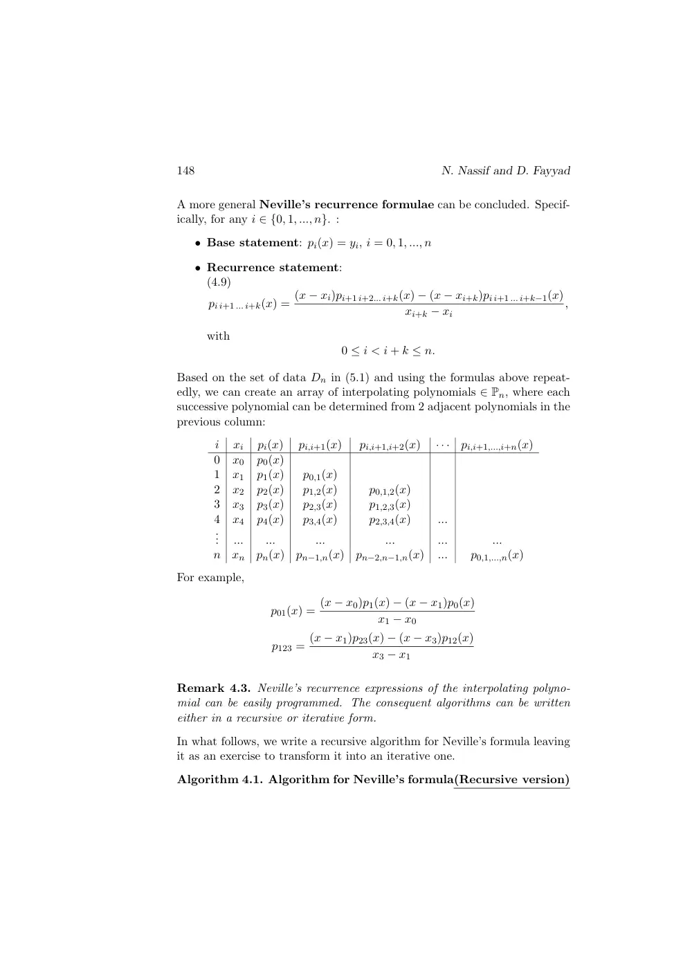
Based on the set of data Dn in (5.1) and using the formulas above repeat-
edly, we can create an array of interpolating polynomials 2 Pn, where each
successive polynomial can be determined from 2 adjacent polynomials in the
previous column:
i
xi
pi(x)
pi,i+1(x)
pi,i+1,i+2(x)
· · ·
pi,i+1,...,i+n(x)
0
x0
p0(x)
1
x1
p1(x)
p0,1(x)
2
x2
p2(x)
p1,2(x)
p0,1,2(x)
3
x3
p3(x)
p2,3(x)
p1,2,3(x)
4
x4
p4(x)
p3,4(x)
p2,3,4(x)
...
...
...
...
...
...
...
...
n
xn
pn(x)
pn−1,n(x)
pn−2,n−1,n(x)
...
p0,1,...,n(x)
For example,
p01(x) = (x − x0)p1(x) − (x − x1)p0(x)
x1 − x0
p123 = (x − x1)p23(x) − (x − x3)p12(x)
x3 − x1
Remark 4.3. Neville’s recurrence expressions of the interpolating polyno-
mial can be easily programmed. The consequent algorithms can be written
either in a recursive or iterative form.
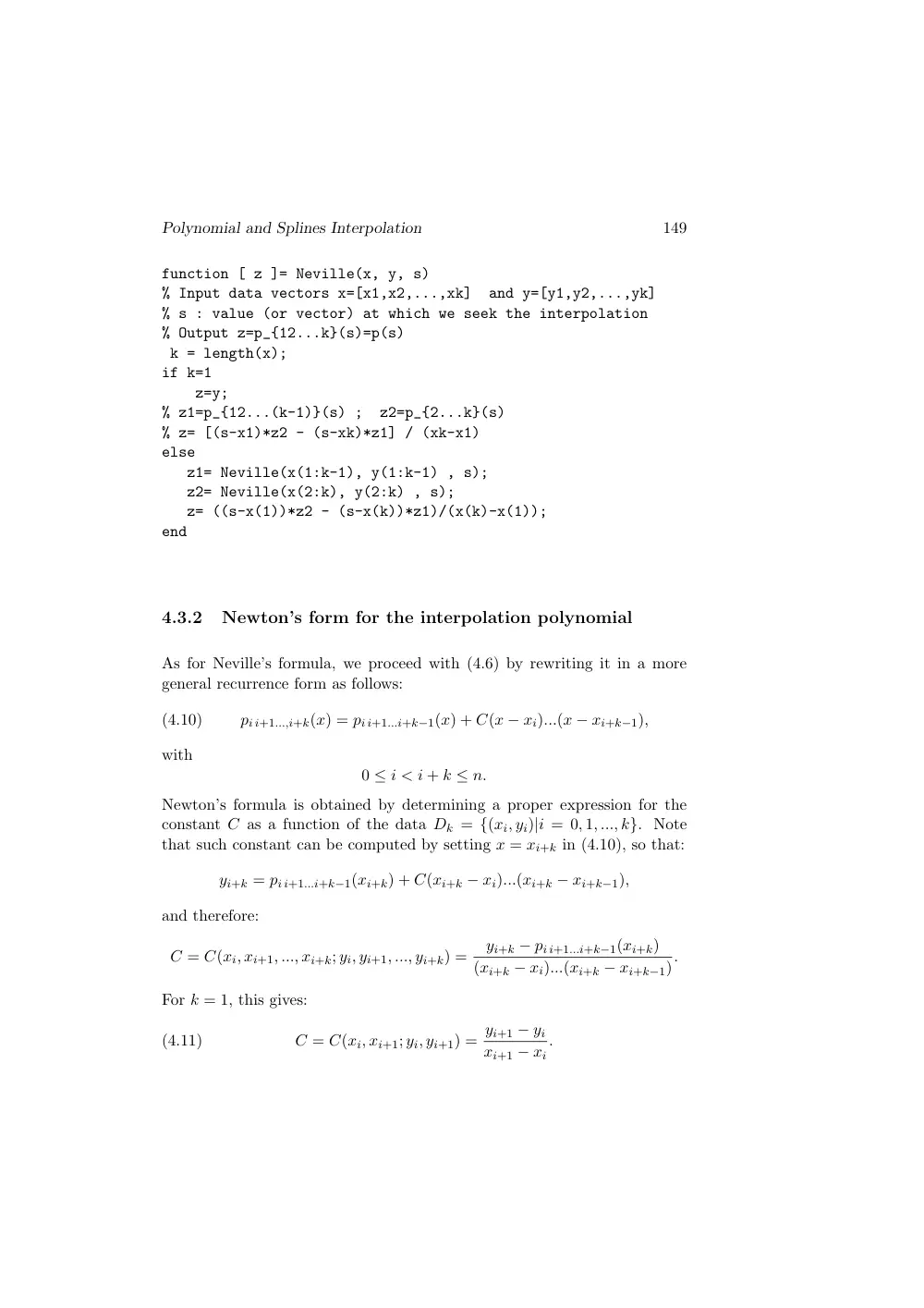
In what follows, we write a recursive algorithm for Neville’s formula leaving
it as an exercise to transform it into an iterative one.
Algorithm 4.1. Algorithm for Neville’s formula(Recursive version)
Polynomial and Splines Interpolation
149
function [ z ]= Neville(x, y, s)
% Input data vectors x=[x1,x2,...,xk]
and y=[y1,y2,...,yk]
% s : value (or vector) at which we seek the interpolation
% Output z=p_{12...k}(s)=p(s)
k = length(x);
if k=1
z=y;
% z1=p_{12...(k-1)}(s) ;
z2=p_{2...k}(s)
% z= [(s-x1)*z2 - (s-xk)*z1] / (xk-x1)
else
z1= Neville(x(1:k-1), y(1:k-1) , s);
z2= Neville(x(2:k), y(2:k) , s);
z= ((s-x(1))*z2 - (s-x(k))*z1)/(x(k)-x(1));
end
4.3.2
Newton’s form for the interpolation polynomial
As for Neville’s formula, we proceed with (4.6) by rewriting it in a more
general recurrence form as follows:
(4.10)
pi i+1...,i+k(x) = pi i+1...i+k−1(x) + C(x − xi)...(x − xi+k−1),
with
0 i < i + k n.
Newton’s formula is obtained by determining a proper expression for the
constant C as a function of the data Dk = {(xi, yi)|i = 0, 1, ..., k}. Note
that such constant can be computed by setting x = xi+k in (4.10), so that:
yi+k = pi i+1...i+k−1(xi+k) + C(xi+k − xi)...(xi+k − xi+k−1),
and therefore:
C = C(xi, xi+1, ..., xi+k; yi, yi+1, ..., yi+k) =
yi+k − pi i+1...i+k−1(xi+k)
(xi+k − xi)...(xi+k − xi+k−1).
For k = 1, this gives:
(4.11)
C = C(xi, xi+1; yi, yi+1) = yi+1 − yi
xi+1 − xi
.
150
N. Nassif and D. Fayyad
Define then
[xi, xi+1] = yi+1 − yi
xi+1 − xi
as the first order divided di↵erence associated with {xi, xi+1}, so that (4.10)
is expressed as follows:
(4.12)
pi,i+1(x) = pi(x) + [xi, xi+1](x − xi)
which is Newton’s formula of order 1. More generally, we may define divided
di↵erences of any order k ≥ 1, through a recurrence process as follows:
Definition 4.1. Given the set of data
Dn = {(xi, yi)|i = 0, 1, ..., n}, xi 6= xj for i 6= j.
Let [xi] = yi, i = 0, 1, ..., n. Then, for 0 i < i + k n, the kth order
divided di↵erence is given through the recurrence formula:
(4.13)
[xi, xi+1, ..., xi+k] = [xi+1, ..., xi+k] − [xi, xi+1, ..., xi+k−1]
xi+k − xi
.
Consequently, we prove that the constant C in (4.10) is a kth order divided
di↵erence. This is done in the following proposition.
Theorem 4.2. Let 0 i < i + k n. Let
pi i+1...i+k(x) = pi i+1...i+k−1(x) + C(x − xi)...(x − xi+k−1),
is the interpolating polynomial based on the nodes {xi, ..., xi+k}, as defined
in (4.6). Then, the constant C is the kth order divided di↵erence
C = [xi, xi+1, ..., xi+k] = [xi+1, ..., xi+k] − [xi, xi+1, ..., xi+k−1]
xi+k − xi
Proof. To obtain this result we use a mathematical induction process on k.
Clearly, (4.12) indicates that the result is true for k = 1.
Assuming now that the proposition is correct for all j k−1 with i+j < n,
then, one writes on the basis of the induction hypothesis for j = k − 1,
successively:
pi...i+k−1(x) = pi...i+k−2(x) + [xi, xi+1, ...xi+k−1](x − xi)...(x − xi+k−2)
where [xi, xi+1, ...xi+k−1] is the coefficient of xk−1 in the polynomial pi...i+k−1(x)
Polynomial and Splines Interpolation
151
and
pi+1...i+k(x) = pi+1, ..., i+k−1(x) + [xi+1, ..., xi+k](x − xi+1)...(x − xi+k−1)
where [xi+1, ..., xi+k] is the coefficient of xk−1 in the polynomial pi+1...i+k(x).
Using now Neville’s formula, one has:
pi...i+k(x) = (x − xi)pi+1...i+k(x) − (x − xi+k)pi...i+k−1(x)
xi+k − xi
.
By equating the coefficients of xk on both sides of this identity one has:
C = [xi+1, ..., xi+k−1, xi+k] − [xi, xi+1, ..., , xi+k−1]
xi+k − xi
,
which is the targeted result of the theorem.
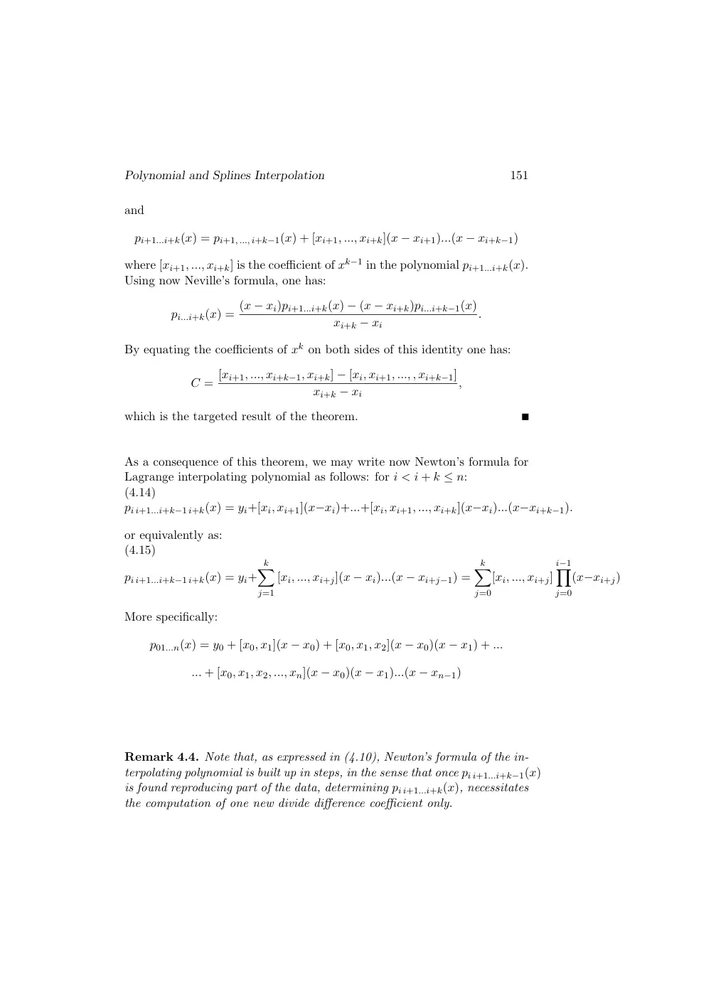
As a consequence of this theorem, we may write now Newton’s formula for
Lagrange interpolating polynomial as follows: for i < i + k n:
(4.14)
pi i+1...i+k−1 i+k(x) = yi+[xi, xi+1](x−xi)+...+[xi, xi+1, ..., xi+k](x−xi)...(x−xi+k−1).
or equivalently as:
(4.15)
pi i+1...i+k−1 i+k(x) = yi+
k
X
j=1
[xi, ..., xi+j](x − xi)...(x − xi+j−1) =
k
X
j=0
[xi, ..., xi+j]
i−1
Y
j=0
(x−xi+j)
More specifically:
p01...n(x) = y0 + [x0, x1](x − x0) + [x0, x1, x2](x − x0)(x − x1) + ...
... + [x0, x1, x2, ..., xn](x − x0)(x − x1)...(x − xn−1)
Remark 4.4. Note that, as expressed in (4.10), Newton’s formula of the in-
terpolating polynomial is built up in steps, in the sense that once pi i+1...i+k−1(x)
is found reproducing part of the data, determining pi i+1...i+k(x), necessitates
the computation of one new divide di↵erence coefficient only.
152
N. Nassif and D. Fayyad
4.3.3
Construction of Divided Di↵erences and Implementa-
tion of Newton’s formula
Let {i0, i1, . . . , ik} of be any permutation of the set of integers {i, i +
1, . . . , i + k}. Based on the uniqueness property of the interpolating polyno-
mials:
pi i+1...i+k−1 i+k(x) = pi0 i1...ik−1 ik(x)
and consequently the kth order divided di↵erences [xi, xi+1, ..., xi+k] and
[xi0, xi1..., xik−1, xik] representing respectively the (same) coefficient of xk in
the two polynomials above, are equal. This leads to the following invariance
property satisfied by divided di↵erences:
Theorem 4.3. Let {i0, i1, . . . , ik} of be any permutation of the set of inte-
gers {i, i + 1, . . . , i + k}. Then:
[xi, xi+1, . . . , xi+k] = [xi0, xi1, . . . , xik]
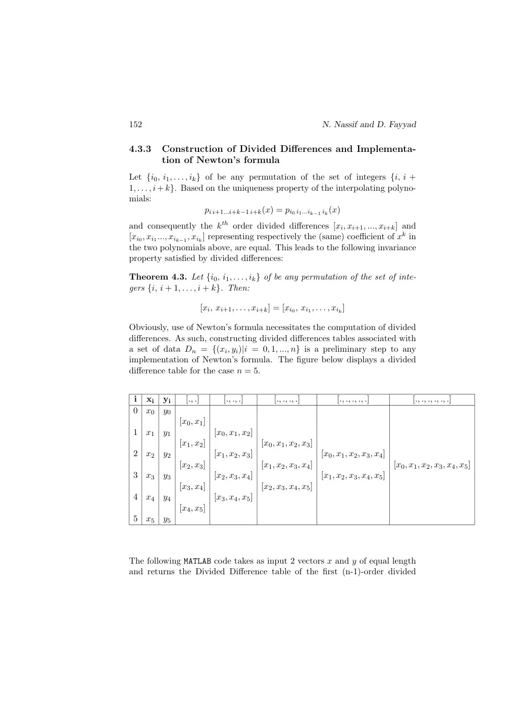
Obviously, use of Newton’s formula necessitates the computation of divided
di↵erences. As such, constructing divided di↵erences tables associated with
a set of data Dn = {(xi, yi)|i = 0, 1, ..., n} is a preliminary step to any
implementation of Newton’s formula. The figure below displays a divided
di↵erence table for the case n = 5.
i
xi
yi
[., .]
[., ., .]
[., ., ., .]
[., ., ., ., .]
[., ., ., ., ., .]
0
x0
y0
[x0, x1]
1
x1
y1
[x0, x1, x2]
[x1, x2]
[x0, x1, x2, x3]
2
x2
y2
[x1, x2, x3]
[x0, x1, x2, x3, x4]
[x2, x3]
[x1, x2, x3, x4]
[x0, x1, x2, x3, x4, x5]
3
x3
y3
[x2, x3, x4]
[x1, x2, x3, x4, x5]
[x3, x4]
[x2, x3, x4, x5]
4
x4
y4
[x3, x4, x5]
[x4, x5]
5
x5
y5
The following MATLAB code takes as input 2 vectors x and y of equal length
and returns the Divided Di↵erence table of the first (n-1)-order divided
Polynomial and Splines Interpolation
153
di↵erences, as a lower triangular matrix, using the MATLAB diff operator.
Algorithm 4.2. Constructing a divided di↵erence table
function D = DivDiffTable(x,y)
% D is a lower Triangular matrix
% If
x=[x(1),x(2),...,x(n)]
is a vector of length n, then :
%
diff(x)=[(x(2)-x(1)), (x(3)-x(2)),....,(x(n)-x(n-1))] is a vector of length (n-1)
n=length(x) ;
m=length(y) ;
if m==n
D=zeros(n,n) ;
D(1:n, 1) = y(1:n) ;
Y= D(1:n, 1)
;
for j=2: n
V1=x(1:n-j+1) ; V2=x(j:n) ;
D(j:n, j)= (diff(Y) ./ (V2-V1)’ ) ;
Y=D(j:n, j) ;
end
end
Example 4.3. Create the Divided Di↵erence Table based on the set of data
of Example 4.2 representing the function f(x) = ln(x):
D5 = {(1, 0) , (1.5, 0.17609) , (2.0, 0.30103) , (3, 0.47712) , (3.5, 0.54407) , (4, 0.60206)}
i
xi
yi
[., .]
[., ., .]
[., ., ., .]
[., ., ., ., .]
[., ., ., ., ., .]
0
1.0
0
0.35218
1
1.5
0.17609
−0.1023
0.24988
0.02655
2
2.0
0.30103
−0.0492
−0.006404
0.17609
0.01054
0.001411
3
3.0
0.47712
−0.02813
−0.002172
0.13390
0.00511
4
3.5
0.54407
−0.01792
0.11598
5
4.0
0.60206
Let us consider now approximations of f(x) for values of x first at the top of
the table, for example x = 1.2, then at the middle of the table, as x = 2.5.
154
N. Nassif and D. Fayyad
(Note that in general, one can prove that the approximation-error is smaller
when x is centered with respect to the nodes).
1. The 1st interpolating polynomials are successively as follows:
• p01(x) = 0.35218(x − 1),
• p012(x) = p01(x) − 0.1023(x − 1)(x − 1.5),
• p0123(x) = p012(x) + 0.02655(x − 1)(x − 1.5)(x − 2),
• p01234(x) = p0123(x) − 0.006404(x − 1)(x − 1.5)(x − 2)(x − 3),
• p012345(x) = p01234(x)+0.001411(x−1)(x−1.5)(x−2)(x−3)(x−3.5).
As a result, approximations to ln(1.2) = 0.0791812460476248 come as
follows:
p...(1.2)
Value
Relative error
p01(x)
0.070436
1.10446 ⇥ 10−1
p012(x)
0.076574
3.2928 ⇥ 10−2
p0123(x)
0.0778484
1.6833 ⇥ 10−2
p01234(x
0.07840171
9.845 ⇥ 10−3
p012345(x)
0.0786821
6.30384 ⇥ 10−3
2. To get approximations to f(2.5),(using Theorem 4.3), we obtain suc-
cessively linear, quadratic and cubic polynomials as follows:
• p23(x) = y2 + [x2, x3](x − x2) = 0.30103 + 0.17609(x − 2)
• p231(x) = p23(x) + [x2, x3, x1](x − x2)(x − x3)
= p23(x) + [x1, x2, x3](x − x2)(x − x3) = p23(x) − 0.0492(x − 2)(x − 3)
• p2314(x) = p231(x) + [x2, x3, x1, x4](x − x2)(x − x3)(x − x1)
= p231(x) + [x1, x2, x3, x4](x − x2)(x − x3)(x − x1) = p231(x) +
0.01054(x − 2)(x − 3)(x − 1.5)
• p2310(x) = p231(x) + [x2, x3, x1, x0](x − x2)(x − x3)(x − x1)
= p231(x) + [x0, x1, x2, x3](x − x2)(x − x3)(x − x1) = p231(x) +
0.02655(x − 2)(x − 3)(x − 1.5)
Another alternative starting with p23(x) would be:
• p234(x) = p23(x) + [x2, x3, x4](x − x2)(x − x3) = p23(x) −
0.02813(x − 2)(x − 3)
• p2345(x) = p234(x) + [x2, x3, x4, x5](x − x2)(x − x3)(x − x4)p234(x) +
0.00511(x − 2)(x − 3)(x − 3.5)
• p2341(x) = p234(x) + [x2, x3, x4, x1](x − x2)(x − x3)(x − x4)
= p234(x)+[x1, x2, x3, x4](x−x2)(x−x3)(x−x4) = p234(x)−0.002172(x−
2)(x − 3)(x − 3.5)
Polynomial and Splines Interpolation
155
This process can be carried through to obtain higher order interpo-
lation polynomials. The following results are obtained for the approx-
imation of ln(2.5) = 0.39794001:
p...(2.5)
Value
Relative error
p23(x)
0.389075
2.227725 ⇥ 10−2
p234(x)
0.3961067
4.6070814 ⇥ 10−3
p231(x)
0.4013733
8.62774435 ⇥ 10−3
p2345(x)
0.3973825
1.4009867 ⇥ 10−3
p2341(x)
0.39874
2.0103315 ⇥ 10−3
Hence, it appears clear that increasing the degree of the interpolation poly-
nomial does not improve much the approximation of the exact value of f(x).
We may now write an algorithm that implements Newton’s formula using
Algorithm 4.2: DivDiffTable(x,y).
Algorithm 4.3. Program for Newton’s formula
function p=NewtonForm(x,y,X)
%Input: two equally sized vectors x and y of length k
%
One vector X of length n
%Output: p(X) based on Newton interpolation formula on the data (x,y)
D=DivDiffTable(x,y);
k=length(x);%(equal to length of y)
n=length(X);X=X(:);
term=ones(n,1);
p=zeros(n,1);
for i=1:k
p=p+D(i,i)*term;
term=term.*(X-x(i));
end
To conclude on recurrence formulae for the Lagrange interpolation polyno-
mial, a rule of thumb would be to use Neville’s formula in case of computer
implementation as it takes only one algorithm to program (Algorithm 4.1).
On the other hand, Newton’s formula requires writing 2 programs: one for
divided di↵erences (Algorithm 4.2) before developing Algorithm 4.3 for a
straightforward evaluation of the interpolation polynomial.
156
N. Nassif and D. Fayyad
4.4
Equally spaced Data: Di↵erence Operators
Consider now the set of data Dn with equidistant x−nodes, i.e.
xi+1 − xi = h, 8i = 0, 1, ..., n − 1.
In this case, we can compute divided di↵erences associated with Dn by using
the “di↵erence functions”
or “di↵erence operators” , based on the
y−data only. Specifically, we make the following definitions:
Definition 4.1. Let Y = [y0, y1, ..., yn], then:
1. ∆1Y = [∆y0, ∆y1, ..., ∆yn−1] is the vector of n first order di↵erences
associated with Y , where ∆yi = yi+1 − yi for i = 0, 1..., n − 1.
2. By recurrence, for k = 2, 3, ...n, we may then define the vector of
kth order di↵erences ∆kY = [∆ky0, ∆ky1, ..., ∆kyn−k], where ∆kyi =
∆k−1yi+1 − ∆k−1yi for i = 0, 1, ..., n − k.
Di↵erence operators are linear in the sense that:
∆k(Y + Z) = ∆kY + ∆kZ and ∆k(aY ) = a∆kY, a 2 R, k = 2, 3, ...n.
Besides, one easily obtains a relation between divided di↵erences and di↵er-
ences of all orders as shown below.
Theorem 4.4. Let Dn be a set of data as defined in (4.1), where the x-nodes
are equally spaced with xi+1 − xi = h, 8i = 0, 1, ..., n − 1. Then for all k
where
1 k with i + k n:
(4.16)
[xi, xi+1, ..., xi+k] = ∆kyi
hkk!
Proof. The proof is done by induction on k. After verifying the result
for k = 1, assume that it is true for 1, ..., k − 1, i.e.:
[xi, xi+1, ..., xi+k−1] =
∆k−1yi
hk−1(k − 1)!.
Since,
[xi, xi+1, ..., xi+k] = [xi+1, ..., xi+k] − [xi, xi+1, ..., xi+k−1]
(xi+k − xi)
,
Polynomial and Splines Interpolation
157
then:
[xi, xi+1, ..., xi+k] =
∆k−1yi+1 − ∆k−1yi
hk−1(k − 1)!(xi+k − xi) = ∆k−1yi+1 − ∆k−1yi
hk−1(k − 1)! kh
.
that reaches the required result.
Based on the theorem above and in case of equally spaced data, Newton’s
interpolating polynomial is expressed as follows::
(4.17)
p(x) = y0+∆y0
1!h (x−x0)+∆2y0
2!h2 (x−x0)(x−x1)+· · ·+∆ny0
n!hn (x−x0)(x−x1) . . . (x−xn−1)
where it is understood that p(x) = p012...n(x).
Remark 4.5. Note the resemblance of this formula with that of Taylor’s
formula for a function f(x) where the nth degree polynomial representing
f(x) is given by:
q(x) = f(x0) + f
0(x0)(x − x0) + .... + f(n)(x0)
n!
(x − x0)n
This remark will be exploited in Chapter 5 when approximating derivatives
such as f(k)(x0) by kth order di↵erences ∆kf(x0)
hn
.
The result of the above theorem allows us therefore to compute divided
di↵erence tables by simply first computing di↵erences as displayed in the
following table:
158
N. Nassif and D. Fayyad
i
xi
yi
∆
∆2
∆3
·
0
x0
y0
∆y0 = y1 − y0
1
x1
y1
∆2y0 = ∆y1 − ∆y0
∆y1 = y2 − y1
∆3y0 = ∆2y1 − ∆2y0
2
x2
y2
∆2y1 = ∆y2 − ∆y1
∆y2 = y3 − y2
...
3
x3
y3
...
...
...
...
...
...
n − 2
xn−2
yn−2
...
∆yn−2 = yn−1 − yn−2
n − 1
xn−1
yn−1
∆2yn−2 = ∆yn−1 − ∆yn−2
∆yn−1 = yn − yn−1
n
xn
yn
Algorithm 4.4. Constructing a di↵erence table
Polynomial and Splines Interpolation
159
Example 4.4. The following set of data D4 is associated with 0-th order
Bessel’s function of the first kind.
i
xi
yi
0
1.0
0.7651977
1
1.3
0.6200860
2
1.6
0.4554022
3
1.9
0.2818186
4
2.2
0.1103623
Since the x-data are equally space with h = 0.3, the di↵erences table can be
easily constructed out of this data:
i
xi
yi
∆
∆2
∆3
∆4
0
1.0
0.7651977
∆y0 = −0.1451117
1
1.3
0.6200860
∆2y0 = −0.0195721
∆y1 = −0.1646838
∆3y0 = 0.0106723
2
1.6
0.4554022
∆2y1 = −0.0088998
∆4y0 = 0.0003548
∆y2 = −0.1735836
∆3y1 = 0.0110271
3
1.9
0.2818186
∆2y2 = 0.0021273
∆y3 = −0.1714563
4
2.2
0.1103623
Using this table, we may subsequently write any of the interpolation poly-
nomials reproducing data in D4. For example:
p234(x) = y2 + ∆y2
0.3 (x − x2) +
∆2y2
(0.3)22!(x − x2)(x − x3)
= 0.4554022 − 0.1735836
0.3
(x − 1.6) + 0.0021273
(0.3)2
(x − 1.6)(x − 1.9)
p231(x) = p23(x) + [x2, x3, x1](x − x2)(x − x3) = p23(x) + [x1, x2, x3](x −
x2)(x − x3)
= p23(x) +
∆2y1
(0.3)22!(x − x2)(x − x3) = p23(x) − 0.0088998
(0.3)22! (x − 1.6)(1 − 1.9)
4.5
Errors in Polynomial Interpolation
When a function f is approximated on an interval [a, b] = [x0, xn] by means
of an interpolating polynomial pn, it is naturally expected that the function
be well approximated at all intermediate points between the nodes, and that
as the number of nodes increases, this agreement will become more and more
160
N. Nassif and D. Fayyad
accurate. Nevertheless, this expectation is wrong and incorrect.
A theoretical estimate of the error is derived in ([20], page 189) and leads
to the following result:
Theorem 4.5. Let f be a function in Cn+1[a, b], and pn the Lagrange poly-
nomial of degree at most n, that interpolates f based on the set of data Dn.
There exists some point c 2 (a, b) such that the error function:
En(f(x)) = f(x) − pn(x) = wn(x)f(n+1)(c)
(n + 1)! ,
where wn(x) = (x − x0)(x − x1)....(x − xn), and x 2 (a, b).
However, such result does not lead to a convergence result in the sense of:
lim
n!1 |f(x) − pn(x)| = 0, 8x 2 (a, b),
even if the function f possesses continuous derivatives of all orders in that
interval.
Example 4.5. A well-known counter example of this phenomenon is pro-
vided by the Runge function:
f(x) =
1
1 + x2
Polynomial and Splines Interpolation
161
Let p01...n(x) be the polynomial that interpolates this function at n + 1
equally spaced nodes on the interval [−5, +5] for example, including the
endpoints. It is easy to verify the following contradictory results:
1. The curve representing p01...n(x) assumes negative values, which obvi-
ously f(x) does not have.
2. Adding more equally spaced nodes, leading to higher degree polyno-
mials worsens the situation. The graphs of the resulting polynomials
have wilder oscillations, especially near the endpoints of the interval,
and the error increases beyond all bounds as confirmed in the graph .
Thus, in this case it can be shown that:
lim
n!1
max
−5x+5 |f(x) − pn(x)| = 1.
This behaviour is called the “Runge’ s phenomenon”.
In a more advanced study of this topic [24], it is proved that the divergence
of the polynomials is often due to the fact that the nodes of interpolation
are equally spaced, which contrary to intuition, is usually a very poor and
inappropriate choice . Specifically, one can show that:
|wn(x)| n!hn+1
4
and therefore
max
x
|f(x) − pn(x)| maxx |f(n+1)(x)|
4(n + 1)
hn+1
If n ! 1, the order of magnitude of maxx |f(n+1)(x)| could outweigh the
nearly-zero order of hn+1/4(n + 1).
In [24], numerical results are conducted in the case of the Runge function
confirming this hypothesis. More specifically, it is verified that
max
−5x+5 |f(22)(x)| = O(1019)
while the corresponding value of max wn(x)
(n+1)! = O(10−10)
A much better and more adequate choice of nodes leading to more accurate
results that help minimizing Runge’ s phenomenon is obtained for example
162
N. Nassif and D. Fayyad
with the set of Chebyshev nodes defined over the unit interval [−1, +1] by:
xi = cos[2i − 1
2n
⇡] , 1 i n
(Note that these values are graphically obtained by projecting equally spaced
points on the unit circle, down on the unit interval [−1, +1]). More generally
over arbitrary interval [a, b] the coordinates of Chebyshev nodes are:
xi = 1
2(a + b) + 1
2(b − a) cos[2i − 1
2n
⇡]
It is possible then to prove that
lim
n!1 |f(x) − pn(x)| = 0
This problem motivates the use of local piecewise polynomial interpolation.
4.6
Local Interpolation: Spline functions
As the global
approach of interpolating polynomials does not provide in
general a systematic and efficient way to approximate a function f(x) on
the basis of the data
Dn = {(xi, yi)|i = 0, 1, ...n, , x0 = a, < x1 < ... < xn−1 < xn = b},
we consider hereafter a local approach that considers approximating a func-
tion f(x) by spline functions. Such functions are piecewise polynomials
joined together with certain imposed “smoothness conditions”.
In the theory of splines, the interior points {xi}n
i=0 at which the function
changes its expression are called the “nodes” or “knots” of the partition.
In this chapter, we analyze successively linear, quadratic and cubic spline
interpolation rather than the global one.
4.6.1
Linear Splines
The simplest connection between two points is a line segment. A spline of
degree one or linear spline, is therefore a function that consists of linear
polynomial pieces joined together to achieve continuity of the polygonal
curve representing it. Its formal definition is given as follows:
Definition 4.2. A linear spline interpolating the data Dn is a function s(x)
such that:
Polynomial and Splines Interpolation
163
1. si(x) = {s(x)|x2[xi,xi+1]} is a polynomial of degree at most 1, i.e.
si 2 P1, 8i = 0, 1, ..., n − 1.
2. s(x) is globally continuous on [a, b], (i.e. s 2 C([a, b], the set of all
continuous functions on [a, b]).
3. s(xi) = yi, 8i = 0, 1, ..., n. (Interpolation conditions)
Note that there exists a unique function s(x) verifying these three criteria:
- To determine s(x), a total of 2n unknowns have to be evaluated as each of
the linear polynomials si(x) defined by the first criterion over the subinter-
val [xi, xi+1] is determined by 2 parameters.
- The second and third criteria impose respectively continuity at the n − 1
interior nodes in addition to the n + 1 interpolation conditions, that add up
to a total of n − 1 + n + 1 = 2n restrictions.
The number of unknown parameters being equal to the number of imposed
conditions, the equations of the linear spline are uniquely determined. We
proceed directly to write them using Newton’s linear interpolating polyno-
mial form on each subinterval [xi, xi+1] | i = 0, 1, ..., n − 1. This gives in a
straightforward way:
(4.18)
si(x) = [xi] + [xi, xi+1](x − xi) = yi + yi+1 − yi
xi+1 − xi
(x − xi), 8i = 0, 1, ..., n − 1.
Clearly, by joining the linear pieces {si(x) |i = 0, 1, ..., −1n}, one obtains the
unique linear spline satisfying the definition above.
The linear spline algorithm is as follows:
Algorithm 4.5. Linear splines
function l = LinearSpline(x, y, r)
% Input: 2 vectors x and y of equal length, and a real number r
% Output: l= s(r): s=linear spline
n=length(x);
% seek i : x(i) < r < x(i+1)
i=max(find(x<r));
% compute l=s(r)=s_i(r)
l=y(i) + (y(i+1)-y(i)) / (x(i+1)-x(i)) * (r-x(i));
Example 4.6. Consider the set of data D4 = {(xi, yi = f(xi)) i = 0, 1, 2, 3, 4}
164
N. Nassif and D. Fayyad
where
i
xi
yi
0
1.0
7.6
1
1.3
2.0
2
1.6
4.5
3
1.9
2.8
4
2.2
11
Determine the linear spline function interpolating D4, then interpolate f(1.4)
1. Given that si(x) = yi + yi+1−yi
xi+1−xi (x − xi):
s0(x) = y0 + y1−y0
x1−x0 (x − x0) = 7.6 − 18.6(x − 1) ; 1.0 x 1.3
s1(x) = y1 + y2−y1
x2−x1 (x − x1) = 2 + 8.3(x − 1.3) ; 1.3 x 1.6
s2(x) = y2 + y3−y2
x3−x2 (x − x2) = 4.5 − 5.6(x − 1.6) ; 1.6 x 1.9
s3(x) = y3 + y4−y3
x4−x3 (x − x3) = 2.8 + 27.3(x − 1.9) ; , 1.9 x 2.2
2. Since x1 < x = 1.4 < x2 ) f(1.4) ⇡ s1(1.4) = 2 + 8.3(1.4 − 1.3) = 2.83
As indicated also by the graph, first order splines are not smooth functions,
the first derivative being discontinuous at each interior node. This deficiency
is overcome by looking at higher order degree splines.
4.6.2
Quadratic Spline Interpolation
We start by providing a definition for interpolating quadratic splines based
on the data Dn.
Definition 4.3. A quadratic spline interpolating the data Dn is a function
s(x) such that:
1. si(x) = {s(x)|x2[xi,xi+1]}, is a polynomial of degree at most 2 , i.e.
si 2 P2, 8i = 0, 1, ..., n − 1.
2. s(x) is globally of class C1, that is:
(a) s 2 C([a, b]),
(b) s0 2 C([a, b]).
3. s(xi) = yi, 8i = 0, 1, ..., n. (Interpolation conditions)
Polynomial and Splines Interpolation
165
In order to determine the equations of the interpolating quadratic spline,
we start by counting