
MATH 251 Notes Chapter 3, Spring 2014
American University of Beirut · Numerical Computing · 40 pages
Showing the first 10 of 40 pages. Download the PDF to see all of it.
More MATH 251 files
Show the text of this notes
Chapter 3
Solving Systems of Linear
Equations By Gaussian
Elimination
3.1
Mathematical Preliminaries
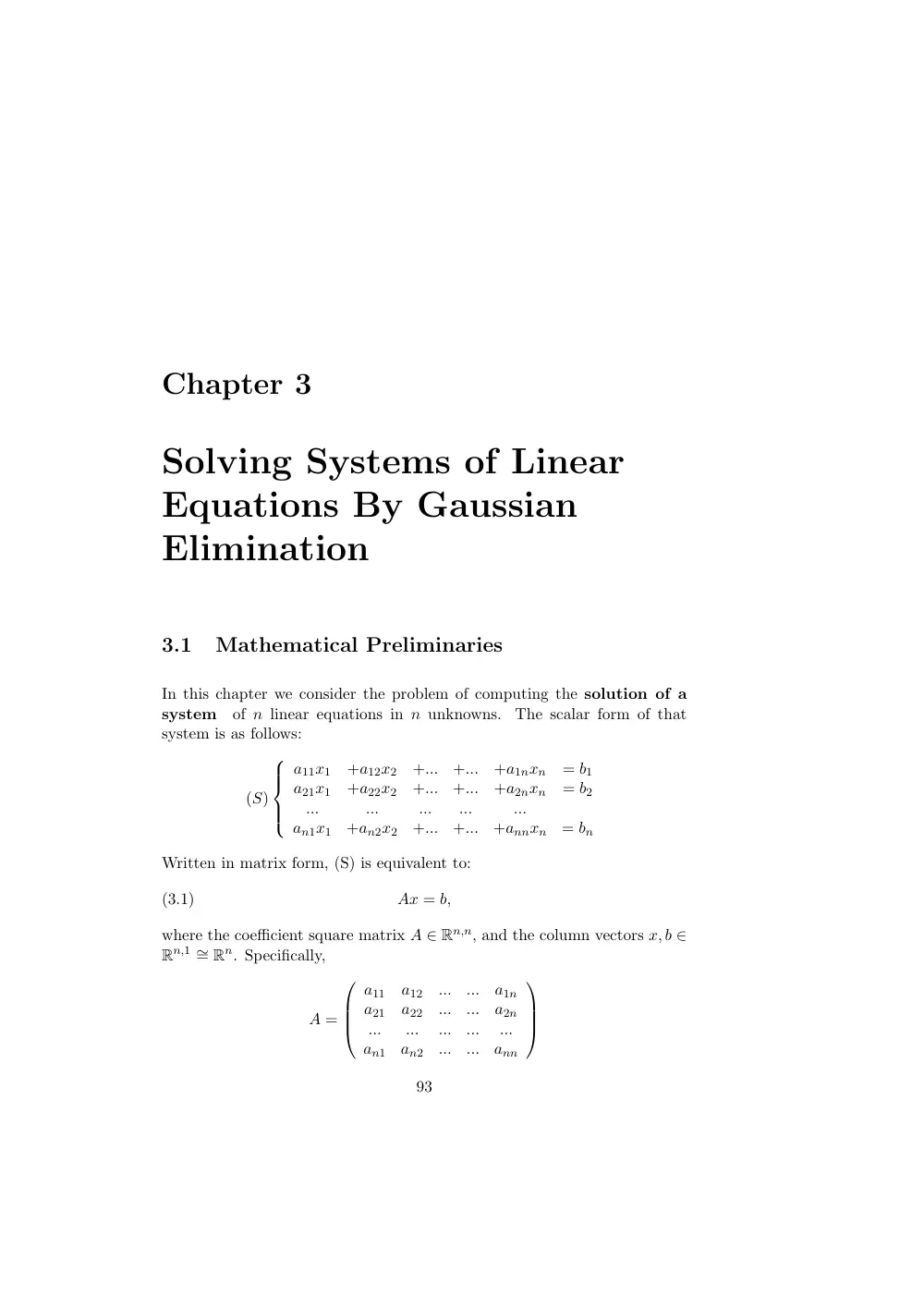
In this chapter we consider the problem of computing the solution of a
system
of n linear equations in n unknowns.
The scalar form of that
system is as follows:
(S)
8
>
>
<
>
>
:
a11x1
+a12x2
+...
+...
+a1nxn
= b1
a21x1
+a22x2
+...
+...
+a2nxn
= b2
...
...
...
...
...
an1x1
+an2x2
+...
+...
+annxn
= bn
Written in matrix form, (S) is equivalent to:
(3.1)
Ax = b,
where the coefficient square matrix A 2 Rn,n, and the column vectors x, b 2
Rn,1 ⇠= Rn. Specifically,
A =
0
B
B
@
a11
a12
...
...
a1n
a21
a22
...
...
a2n
...
...
...
...
...
an1
an2
...
...
ann
1
C
C
A
93
94
N. Nassif and D. Fayyad
x =
0
B
B
@
x1
x2
...
xn
1
C
C
A and b =
0
B
B
@
b1
b2
...
bn
1
C
C
A .
We assume that the basic linear algebra property for systems of linear equa-
tions like (3.1) are satisfied. Specifically:
Proposition 3.1. The following statements are equivalent:
1. System (3.1) has a unique solution.
2. det(A) 6= 0.
3. A is invertible.
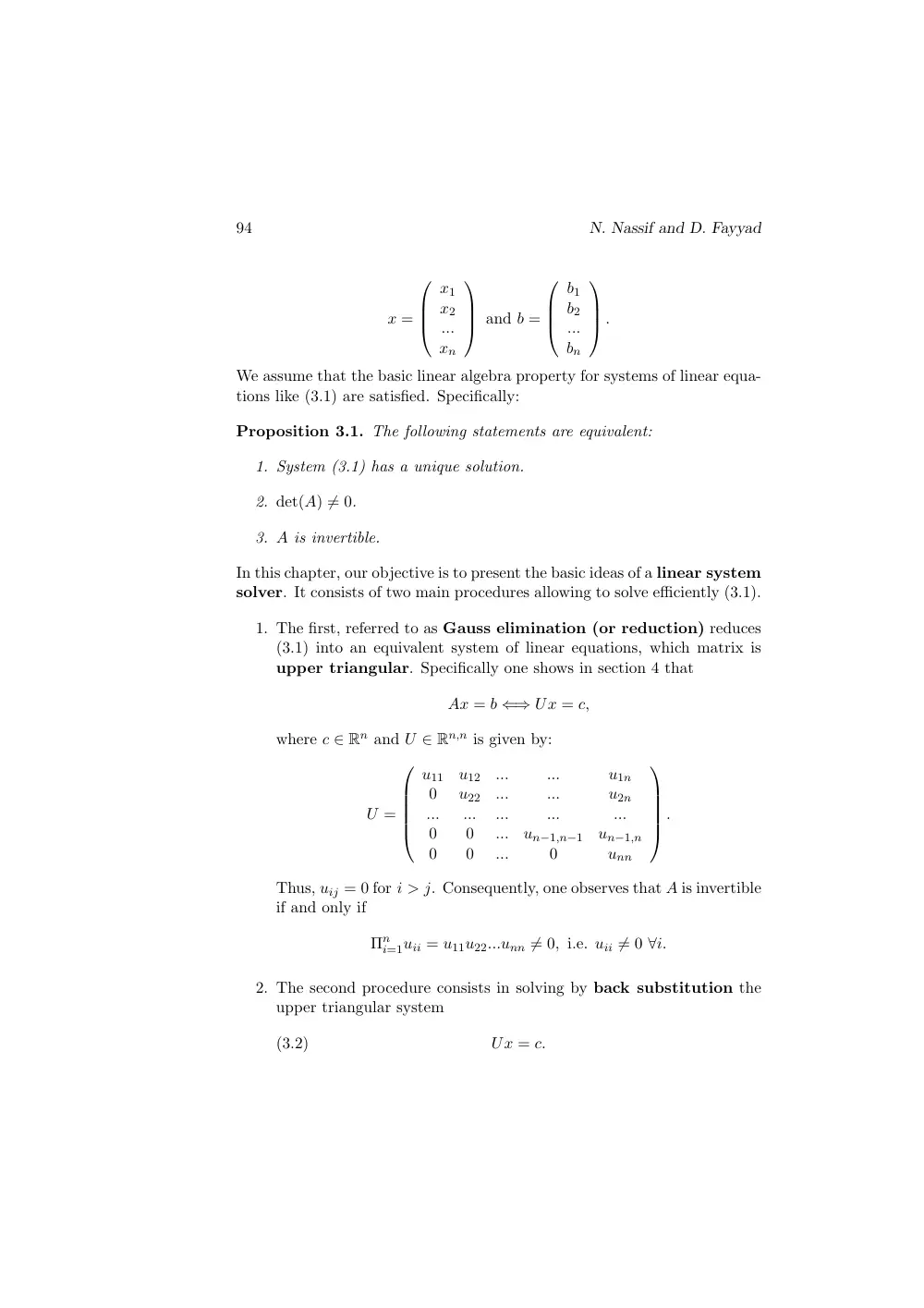
In this chapter, our objective is to present the basic ideas of a linear system
solver. It consists of two main procedures allowing to solve efficiently (3.1).
1. The first, referred to as Gauss elimination (or reduction) reduces
(3.1) into an equivalent system of linear equations, which matrix is
upper triangular. Specifically one shows in section 4 that
Ax = b () Ux = c,
where c 2 Rn and U 2 Rn,n is given by:
U =
0
B
B
B
B
@
u11
u12
...
...
u1n
0
u22
...
...
u2n
...
...
...
...
...
0
0
...
un−1,n−1
un−1,n
0
0
...
0
unn
1
C
C
C
C
A
.
Thus, uij = 0 for i > j. Consequently, one observes that A is invertible
if and only if
⇧n
i=1uii = u11u22...unn 6= 0, i.e. uii 6= 0 8i.
2. The second procedure consists in solving by back substitution the
upper triangular system
(3.2)
Ux = c.
Gaussian Elimination for linear systems
95
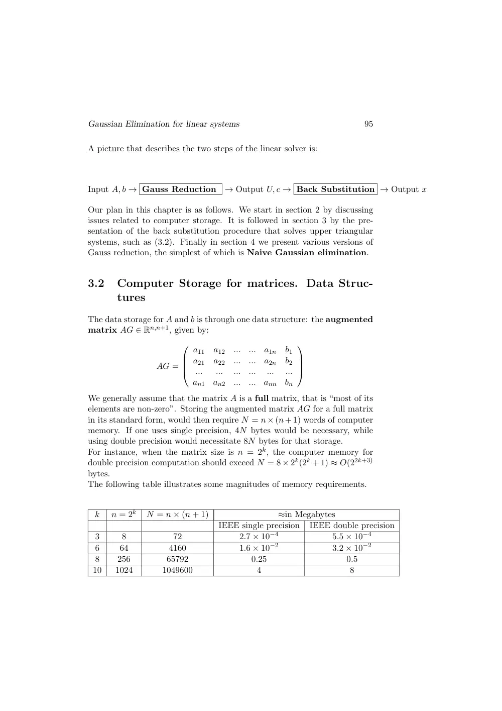
A picture that describes the two steps of the linear solver is:
Input A, b ! Gauss Reduction
! Output U, c ! Back Substitution ! Output x
Our plan in this chapter is as follows. We start in section 2 by discussing
issues related to computer storage. It is followed in section 3 by the pre-
sentation of the back substitution procedure that solves upper triangular
systems, such as (3.2). Finally in section 4 we present various versions of
Gauss reduction, the simplest of which is Naive Gaussian elimination.
3.2
Computer Storage for matrices. Data Struc-
tures
The data storage for A and b is through one data structure: the augmented
matrix AG 2 Rn,n+1, given by:
AG =
0
B
B
@
a11
a12
...
...
a1n
b1
a21
a22
...
...
a2n
b2
...
...
...
...
...
...
an1
an2
...
...
ann
bn
1
C
C
A
We generally assume that the matrix A is a full matrix, that is “most of its
elements are non-zero”. Storing the augmented matrix AG for a full matrix
in its standard form, would then require N = n⇥(n+1) words of computer
memory. If one uses single precision, 4N bytes would be necessary, while
using double precision would necessitate 8N bytes for that storage.
For instance, when the matrix size is n = 2k, the computer memory for
double precision computation should exceed N = 8 ⇥ 2k(2k + 1) ⇡ O(22k+3)
bytes.
The following table illustrates some magnitudes of memory requirements.
k
n = 2k
N = n ⇥ (n + 1)
⇡in Megabytes
IEEE single precision
IEEE double precision
3
8
72
2.7 ⇥ 10−4
5.5 ⇥ 10−4
6
64
4160
1.6 ⇥ 10−2
3.2 ⇥ 10−2
8
256
65792
0.25
0.5
10
1024
1049600
4
8
96
N. Nassif and D. Fayyad
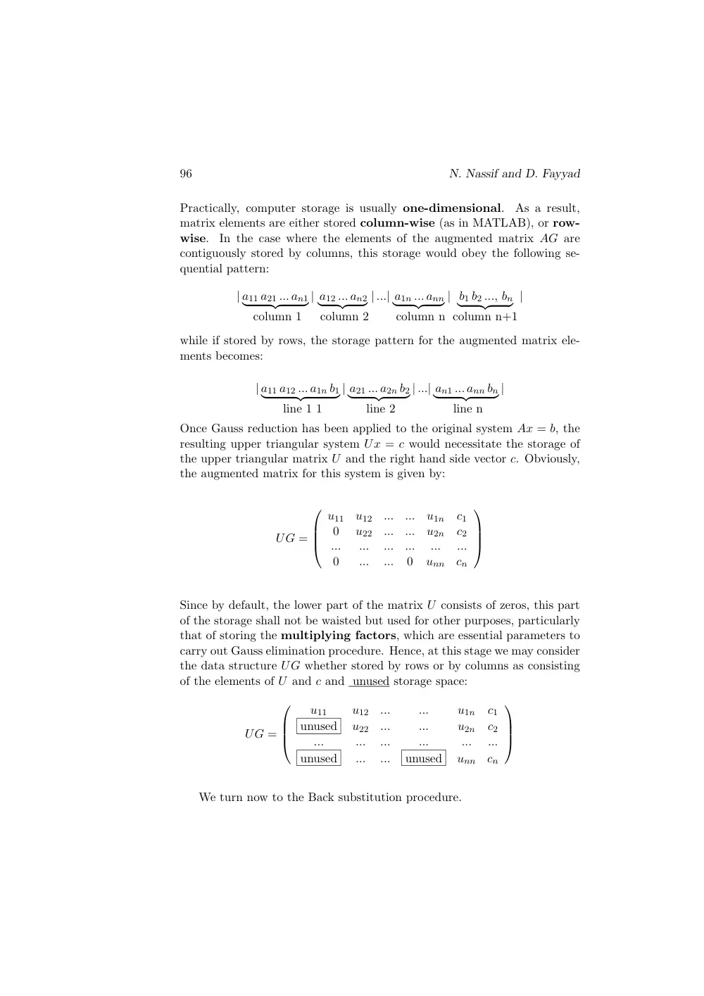
Practically, computer storage is usually one-dimensional.
As a result,
matrix elements are either stored column-wise (as in MATLAB), or row-
wise.
In the case where the elements of the augmented matrix AG are
contiguously stored by columns, this storage would obey the following se-
quential pattern:
| a11 a21 ... an1
|
{z
}
column 1
| a12 ... an2
|
{z
}
column 2
| ...| a1n ... ann
|
{z
}
column n
| b1 b2 ..., bn
|
{z
}
column n+1
|
while if stored by rows, the storage pattern for the augmented matrix ele-
ments becomes:
| a11 a12 ... a1n b1
|
{z
}
line 1 1
| a21 ... a2n b2
|
{z
}
line 2
| ...| an1 ... ann bn
|
{z
}
line n
|
Once Gauss reduction has been applied to the original system Ax = b, the
resulting upper triangular system Ux = c would necessitate the storage of
the upper triangular matrix U and the right hand side vector c. Obviously,
the augmented matrix for this system is given by:
UG =
0
B
B
@
u11
u12
...
...
u1n
c1
0
u22
...
...
u2n
c2
...
...
...
...
...
...
0
...
...
0
unn
cn
1
C
C
A
Since by default, the lower part of the matrix U consists of zeros, this part
of the storage shall not be waisted but used for other purposes, particularly
that of storing the multiplying factors, which are essential parameters to
carry out Gauss elimination procedure. Hence, at this stage we may consider
the data structure UG whether stored by rows or by columns as consisting
of the elements of U and c and unused storage space:
UG =
0
B
B
@
u11
u12
...
...
u1n
c1
unused
u22
...
...
u2n
c2
...
...
...
...
...
...
unused
...
...
unused
unn
cn
1
C
C
A
We turn now to the Back substitution procedure.
Gaussian Elimination for linear systems
97
3.3
Back Substitution for Upper Triangular Sys-
tems
Although this procedure comes after the completion of the Gauss Reduction
step, we shall deal with it from the start. It indeed provides the importance
of this global approach.
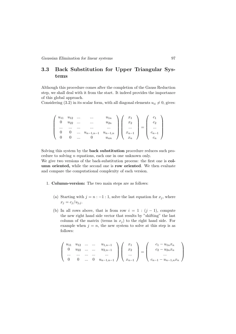
Considering (3.2) in its scalar form, with all diagonal elements uii 6= 0, gives:
0
B
B
B
B
@
u11
u12
...
...
u1n
0
u22
...
...
u2n
...
...
...
...
...
0
0
...
un−1,n−1
un−1,n
0
0
...
0
unn
1
C
C
C
C
A
0
B
B
B
B
@
x1
x2
...
xn−1
xn
1
C
C
C
C
A
=
0
B
B
B
B
@
c1
c2
...
cn−1
cn
1
C
C
C
C
A
Solving this system by the back substitution procedure reduces such pro-
cedure to solving n equations, each one in one unknown only.
We give two versions of the back-substitution process: the first one is col-
umn oriented, while the second one is row oriented. We then evaluate
and compare the computational complexity of each version.
1. Column-version: The two main steps are as follows:
(a) Starting with j = n : −1 : 1, solve the last equation for xj, where
xj = cj/uj,j.
(b) In all rows above, that is from row i = 1 : (j − 1), compute
the new right hand side vector that results by ”shifting” the last
column of the matrix (terms in xj) to the right hand side. For
example when j = n, the new system to solve at this step is as
follows:
0
B
B
@
u11
u12
...
...
u1,n−1
0
u22
...
...
u2,n−1
...
...
...
...
...
0
0
...
0
un−1,n−1
1
C
C
A
0
B
B
@
x1
x2
...
xn−1
1
C
C
A =
0
B
B
@
c1 − u1nxn
c2 − u2nxn
...
cn−1 − un−1,nxn
1
C
C
A
98
N. Nassif and D. Fayyad
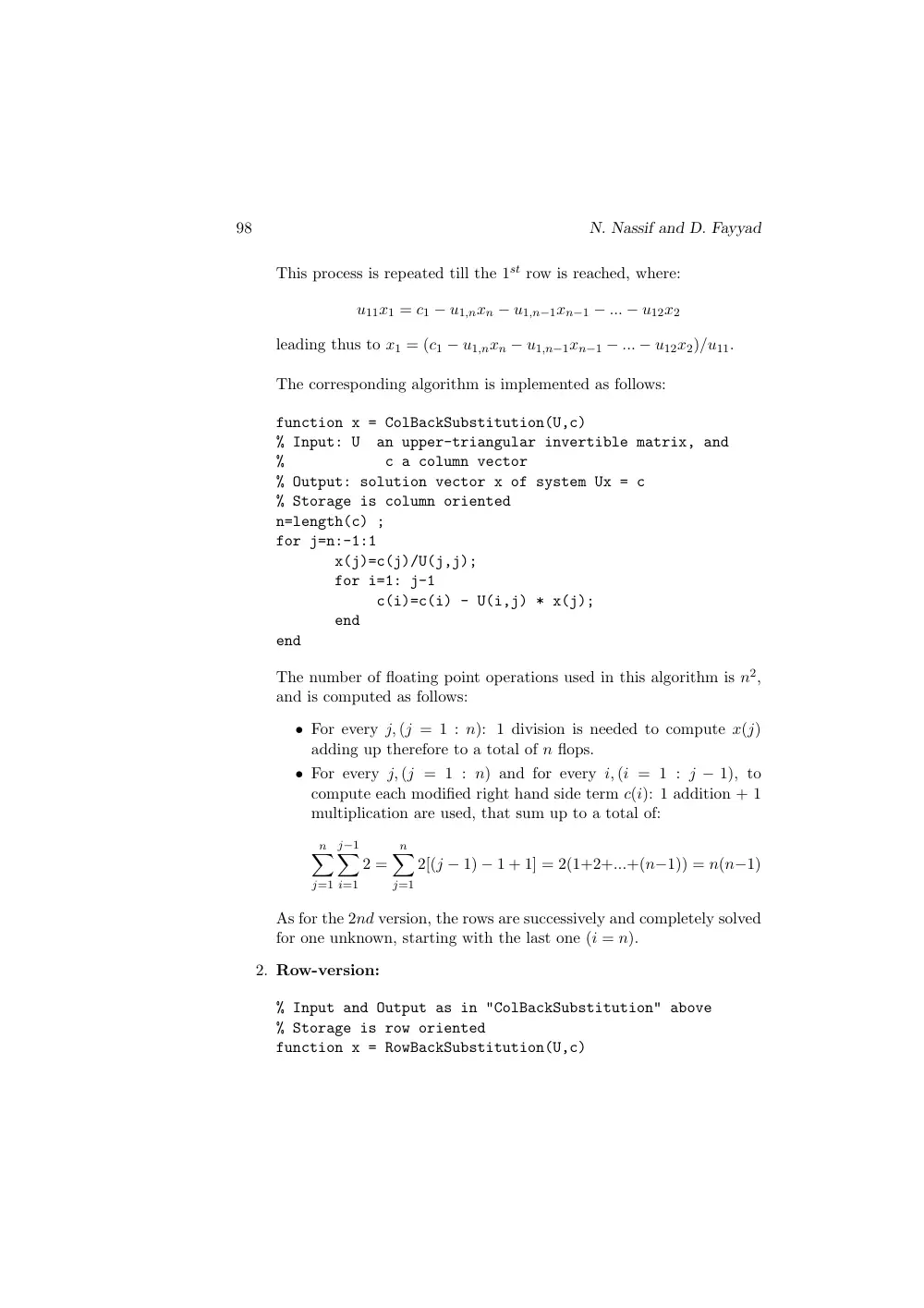
This process is repeated till the 1st row is reached, where:
u11x1 = c1 − u1,nxn − u1,n−1xn−1 − ... − u12x2
leading thus to x1 = (c1 − u1,nxn − u1,n−1xn−1 − ... − u12x2)/u11.
The corresponding algorithm is implemented as follows:
function x = ColBackSubstitution(U,c)
% Input: U
an upper-triangular invertible matrix, and
%
c a column vector
% Output: solution vector x of system Ux = c
% Storage is column oriented
n=length(c) ;
for j=n:-1:1
x(j)=c(j)/U(j,j);
for i=1: j-1
c(i)=c(i) - U(i,j) * x(j);
end
end
The number of floating point operations used in this algorithm is n2,
and is computed as follows:
• For every j, (j = 1 : n): 1 division is needed to compute x(j)
adding up therefore to a total of n flops.
• For every j, (j = 1 : n) and for every i, (i = 1 : j − 1), to
compute each modified right hand side term c(i): 1 addition + 1
multiplication are used, that sum up to a total of:
n
X
j=1
j−1
X
i=1
2 =
n
X
j=1
2[(j − 1) − 1 + 1] = 2(1+2+...+(n−1)) = n(n−1)
As for the 2nd version, the rows are successively and completely solved
for one unknown, starting with the last one (i = n).
2. Row-version:
% Input and Output as in "ColBackSubstitution" above
% Storage is row oriented
function x = RowBackSubstitution(U,c)
Gaussian Elimination for linear systems
99
n=length(c);
x(n)=c(n)/U(n,n);
for i=n-1:-1:1
for j=i+1:n
c(i)=c(i)-U(i,j) * x(j);
end
x(i)=c(i)/U(i,i);
end
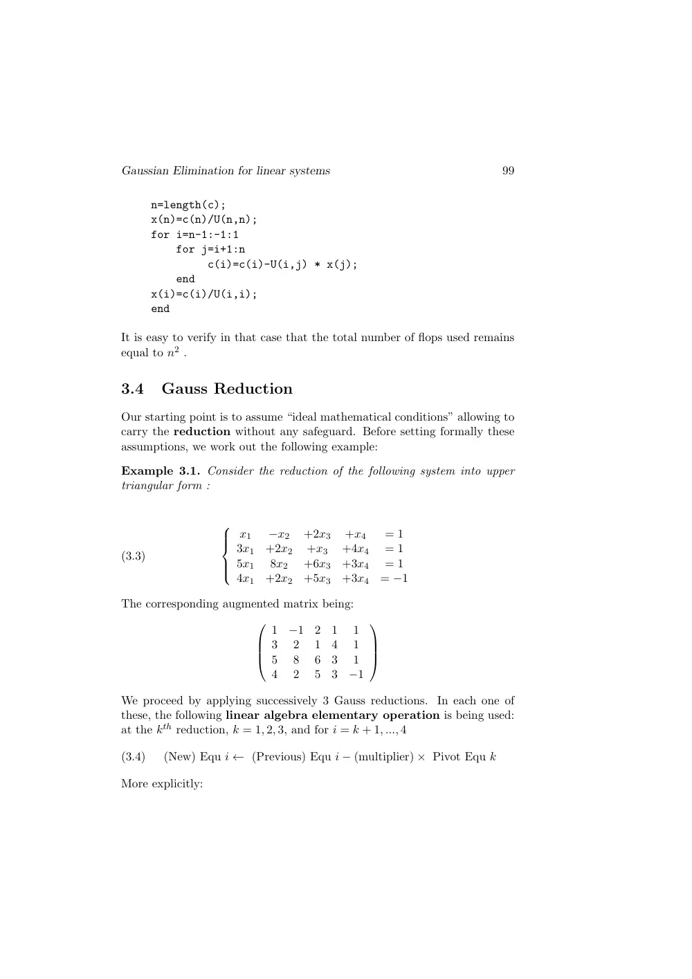
It is easy to verify in that case that the total number of flops used remains
equal to n2 .
3.4
Gauss Reduction
Our starting point is to assume “ideal mathematical conditions” allowing to
carry the reduction without any safeguard. Before setting formally these
assumptions, we work out the following example:
Example 3.1. Consider the reduction of the following system into upper
triangular form :
(3.3)
8
>
>
<
>
>
:
x1
−x2
+2x3
+x4
= 1
3x1
+2x2
+x3
+4x4
= 1
5x1
8x2
+6x3
+3x4
= 1
4x1
+2x2
+5x3
+3x4
= −1
The corresponding augmented matrix being:
0
B
B
@
1
−1
2
1
1
3
2
1
4
1
5
8
6
3
1
4
2
5
3
−1
1
C
C
A
We proceed by applying successively 3 Gauss reductions. In each one of
these, the following linear algebra elementary operation is being used:
at the kth reduction, k = 1, 2, 3, and for i = k + 1, ..., 4
(3.4)
(New) Equ i (Previous) Equ i − (multiplier) ⇥ Pivot Equ k
More explicitly:
100
N. Nassif and D. Fayyad
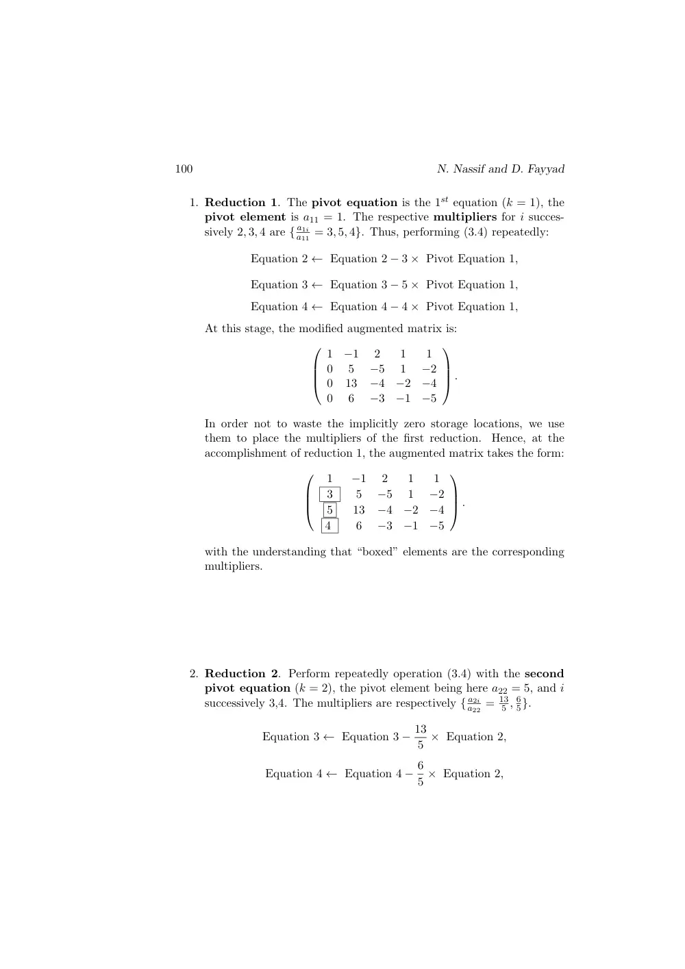
1. Reduction 1. The pivot equation is the 1st equation (k = 1), the
pivot element is a11 = 1. The respective multipliers for i succes-
sively 2, 3, 4 are { a1i
a11 = 3, 5, 4}. Thus, performing (3.4) repeatedly:
Equation 2 Equation 2 − 3 ⇥ Pivot Equation 1,
Equation 3 Equation 3 − 5 ⇥ Pivot Equation 1,
Equation 4 Equation 4 − 4 ⇥ Pivot Equation 1,
At this stage, the modified augmented matrix is:
0
B
B
@
1
−1
2
1
1
0
5
−5
1
−2
0
13
−4
−2
−4
0
6
−3
−1
−5
1
C
C
A .
In order not to waste the implicitly zero storage locations, we use
them to place the multipliers of the first reduction.
Hence, at the
accomplishment of reduction 1, the augmented matrix takes the form:
0
B
B
@
1
−1
2
1
1
3
5
−5
1
−2
5
13
−4
−2
−4
4
6
−3
−1
−5
1
C
C
A .
with the understanding that “boxed” elements are the corresponding
multipliers.
2. Reduction 2. Perform repeatedly operation (3.4) with the second
pivot equation (k = 2), the pivot element being here a22 = 5, and i
successively 3,4. The multipliers are respectively { a2i
a22 = 13
5 , 6
5}.
Equation 3 Equation 3 − 13
5 ⇥ Equation 2,
Equation 4 Equation 4 − 6
5 ⇥ Equation 2,
Gaussian Elimination for linear systems
101
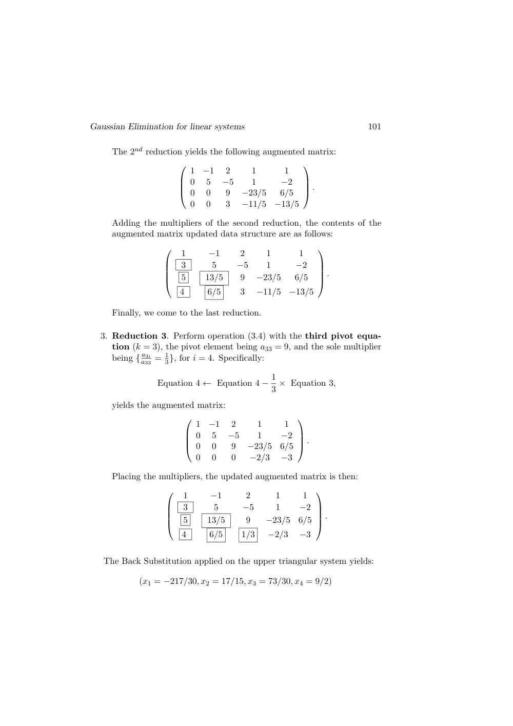
The 2nd reduction yields the following augmented matrix:
0
B
B
@
1
−1
2
1
1
0
5
−5
1
−2
0
0
9
−23/5
6/5
0
0
3
−11/5
−13/5
1
C
C
A .
Adding the multipliers of the second reduction, the contents of the
augmented matrix updated data structure are as follows:
0
B
B
B
@
1
−1
2
1
1
3
5
−5
1
−2
5
13/5
9
−23/5
6/5
4
6/5
3
−11/5
−13/5
1
C
C
C
A .
Finally, we come to the last reduction.
3. Reduction 3. Perform operation (3.4) with the third pivot equa-
tion (k = 3), the pivot element being a33 = 9, and the sole multiplier
being { a3i
a33 = 1
3}, for i = 4. Specifically:
Equation 4 Equation 4 − 1
3 ⇥ Equation 3,
yields the augmented matrix:
0
B
B
@
1
−1
2
1
1
0
5
−5
1
−2
0
0
9
−23/5
6/5
0
0
0
−2/3
−3
1
C
C
A .
Placing the multipliers, the updated augmented matrix is then:
0
B
B
B
@
1
−1
2
1
1
3
5
−5
1
−2
5
13/5
9
−23/5
6/5
4
6/5
1/3
−2/3
−3
1
C
C
C
A .
The Back Substitution applied on the upper triangular system yields:
(x1 = −217/30, x2 = 17/15, x3 = 73/30, x4 = 9/2)
102
N. Nassif and D. Fayyad
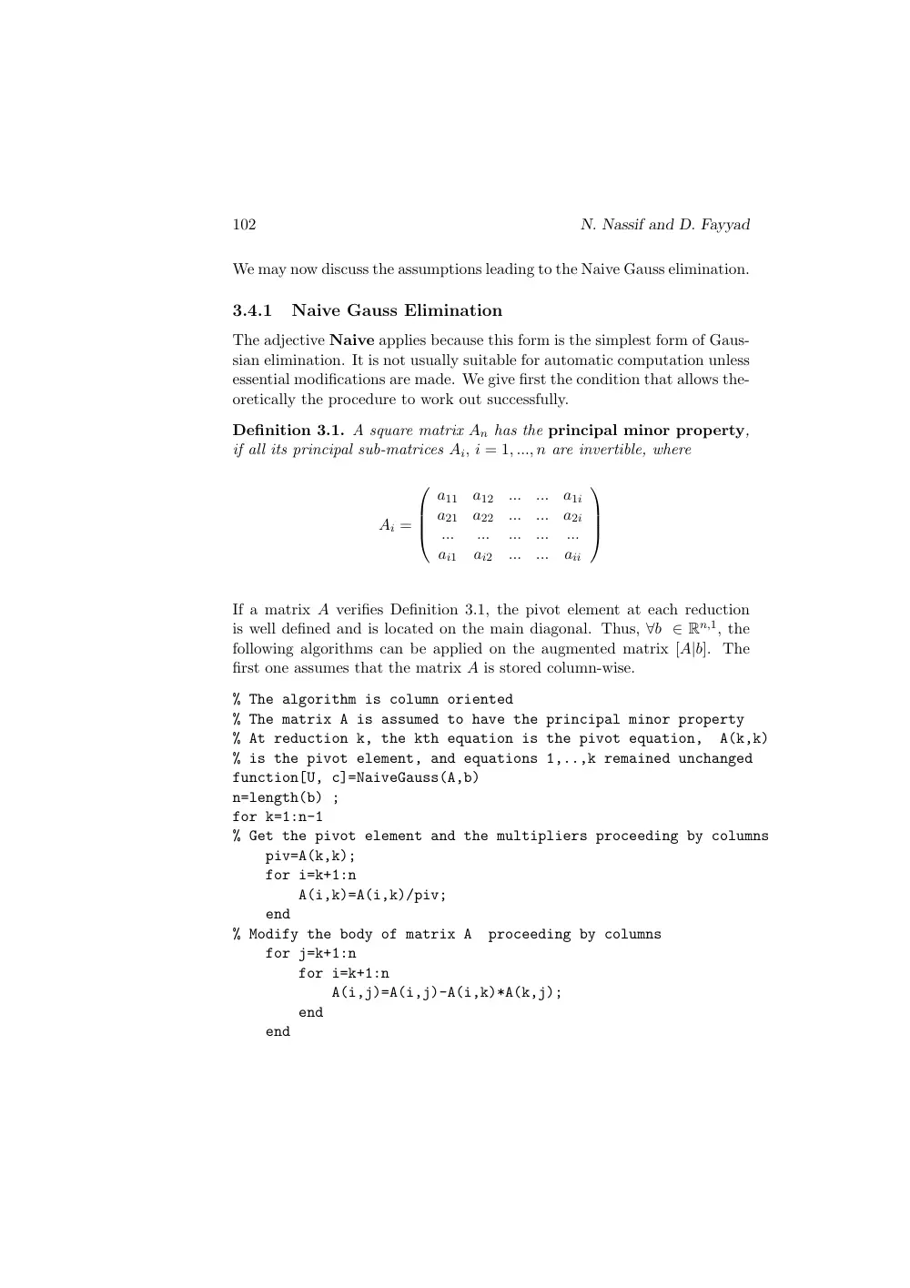
We may now discuss the assumptions leading to the Naive Gauss elimination.
3.4.1
Naive Gauss Elimination
The adjective Naive applies because this form is the simplest form of Gaus-
sian elimination. It is not usually suitable for automatic computation unless
essential modifications are made. We give first the condition that allows the-
oretically the procedure to work out successfully.
Definition 3.1. A square matrix An has the principal minor property,
if all its principal sub-matrices Ai, i = 1, ..., n are invertible, where
Ai =
0
B
B
@
a11
a12
...
...
a1i
a21
a22
...
...
a2i
...
...
...
...
...
ai1
ai2
...
...
aii
1
C
C
A
If a matrix A verifies Definition 3.1, the pivot element at each reduction
is well defined and is located on the main diagonal. Thus, 8b 2 Rn,1, the
following algorithms can be applied on the augmented matrix [A|b]. The
first one assumes that the matrix A is stored column-wise.
% The algorithm is column oriented
% The matrix A is assumed to have the principal minor property
% At reduction k, the kth equation is the pivot equation,
A(k,k)
% is the pivot element, and equations 1,..,k remained unchanged
function[U, c]=NaiveGauss(A,b)
n=length(b) ;
for k=1:n-1
% Get the pivot element and the multipliers proceeding by columns
piv=A(k,k);
for i=k+1:n
A(i,k)=A(i,k)/piv;
end
% Modify the body of matrix A
proceeding by columns
for j=k+1:n
for i=k+1:n
A(i,j)=A(i,j)-A(i,k)*A(k,j);
end
end
Gaussian Elimination for linear systems
103
% Modify the right hand side b
for i=k+1:n
b(i)=b(i)-A(i,k)*b(k);
end
end
% Extract c and U proceeding by columns
c=b;
U=triu(A);
The flop count for this algorithm can be easily evaluated:
1. To find the multipliers:
n−1
X
k=1
n
X
i=k+1
1 =
n−1
X
k=1
n − k = 1 + 2 + ... + (n − 1) = n(n − 1)
2
divisions
2. To modify the body of the matrix:
n−1
X
k=1
n
X
j=k+1
n
X
i=k+1
2 =
n−1
X
k=1
n
X
j=k+1
2(n − k) = 2
n−1
X
k=1
(n − k)2 = 2[12+22+...+(n−1)2]
= 2
h
n(n−1)(2n−1)
6
i
operations.
3. To modify the right hand side vector:
n−1
X
k=1
n
X
i=k+1
2 = 2
n−1
X
k=1
n − k = 2[1+2+...+(n−1)] = 2
n(n − 1)
2
�
operations
In term of flops, this would total to:
n(n − 1)
2
+ n(n − 1)(2n − 1)
3
+ n(n − 1) = n(n − 1)
6
(7 + 4n) = O(2n3
3 ).
The next version requires the same number of flops but is row oriented
% The algorithm is row oriented
% The matrix A is assumed to have the principal minor property
% At reduction k, the kth equation is the pivot equation and A(k,k)
% is the pivot element, and equations 1,..,k remained unchanged
function[c,U]=naiveGauss(A,b)
n=length(b) ;
104
N. Nassif and D. Fayyad
for k=1:n-1
% Get the pivot element
piv=A(k,k);
% Proceed by row: get the multiplier for equation i
for i=k+1:n
A(i,k)=A(i,k)/piv;
% and modify its remaining coefficients, then its right hand side
for j=k+1:n
A(i,j)=A(i,j)-A(i,k)*A(k,j);
end
b(i)=b(i)-A(i,k)*b(k);
end
end
% Extract c and U
c=b;
U=triu(A);
The above 2 versions that are the simplest expressions of Gaussian elimi-
nation, do not take into account the eventual sensitivity of the system to
propagate round-o↵ errors.
3.4.2
Partial Pivoting strategies: Unscaled (Simple) and Scaled
Partial Pivoting
When computing in floating point systems F, there are several situations
where the application of the Naive Gaussian elimination algorithms fails
although the matrix A may verify the principal minor property.
As an illustration consider first the case where the pivot element is relatively
small in F. This would lead to large multipliers that worsen the round-o↵
errors, as shown in the following example.
Example 3.2. Consider the following 2 ⇥ 2 system of equations, where ✏ is
a small non zero number:
(3.5)
⇢ ✏x1 + x2 = 2
3x1 + x2 = 1
The exact solution to this problem in R is x1 ⇡ −1
3 and x2 ⇡ 2.
Gaussian Elimination for linear systems
105
Naive Gauss elimination where the pivot is ✏ leads to:
⇢
✏x1 + x2 = 1
(1 − 3
✏)x2 = 1 − 6
✏
and the back substitution procedure would give:
(
x2 = 1−6/✏
1−3/✏
x1 = 2−x2
✏
If these calculations are performed in a floating point system F, as 1/✏ is
large, then
⇢ 1 − 6
✏ ⇡ − 6
✏
1 − 3
✏ ⇡ − 3
✏
The computed solutions in that case are incorrect, with:
x2 ⇡ 2 and x1 ⇡ 0.
However, if we perform a permutation of the equations before the reduction
process, then the equivalent system becomes :
⇢ 3x1 + x2 = 1
✏x1 + x2 = 2
Carried out, Naive Gauss reduction would lead to:
⇢
3x1 + x2 = 1
(1 − ✏
3)x2 = 2 − ✏
3
Back substitution in this case would clearly give: x2 ⇡ 2 and x1 ⇡ −1/3.
This example leads us to conclude that some type of strategy is essential
for selecting new pivot equations and new pivots at each Gaussian reduc-
tion. Theoretically Complete Pivoting would be the best approach. This
process requires at each stage, first searching over all entries of adequate
submatrices - in all rows and all columns - for the largest entry in absolute
value and then permuting rows and columns to move that entry into the
required pivot position. This would be quite expensive as a great amount
of searching and data movement would be involved. However, scanning just
the 1st column in the submatrix at each reduction and selecting as pivot the
greatest absolute value entry accomplishes our goal, thus avoiding too small
106
N. Nassif and D. Fayyad
or zero pivots. This is Unscaled (or Simple) Partial Pivoting. It would
solve the posed problem, but compared to Complete Pivoting strategy, it
does not involve an examination of the entries in the rows of the matrix.
Moreover, rather than interchanging rows through the this partial pivoting
procedure, that is to avoid the data movement, we use an indexing array.
Thus, the order in which the equations are used is denoted by the row vec-
tor IV called the Index Vector. At first, IV is set to [1, 2, ..., n], then at
each reduction, if there would be a permutation in the rows, it is performed
only on IV which acts as a vector of pointers to the memory location of the
rows. In fact, at each reduction, IV=[i1, i2, ..., in] which is a permutation
of the initial vector IV. This definitely eliminates the time consuming and
unnecessary process of moving around the coefficients of equations in the
computer memory.
We formalize now the Unscaled Partial Pivoting procedure.
1. Gaussian Elimination with Unscaled Partial Pivoting
This strategy consists in first finding at reduction k, the ”best” pivot
equation. This is achieved by identifying the maximum absolute value
element in the kth column, located in some row ranging from the kth
row to the last. More explicitly:
- At reduction k = 1 , seek i1 in the set {1, 2, ..., n} such that:
|ai1,1| = max
1in |ai1| = max {|a11|, |a21|, ..., |an1|}
then perform a permutation of row 1 and row i1 in IV only. Row i1
is the first pivot equation, and ai1,1 is the pivot element. We write
IV ([1, i1]) = IV ([i1, 1]), meaning that at this stage,
IV = [i1, ..., 1, ..., n] = [i1, i2, ..., in]
- At reduction k, seek ik in {IV (k), ..., IV (n)}, such that:
|aik,k| =
max
IV (k)iIV (n) |aik| = max
�
|aIV (k),k|, |aIV (k+1),k|, ..., |aIV (n),k|
repositioning ik in IV will set ik = ik + (k − 1), so that row IV (ik) is
the pivot equation and aIV (ik),k is the pivot element. Perform then a
permutation of rows IV (k) and IV (ik)) in the last IV. Therefore one
writes:
IV ([k, ik]) = IV ([ik, k])
Gaussian Elimination for linear systems
107
As such, in case of e↵ective row permutation, the Naive Gauss Elimi-
nation algorithm is modified as follows:
% The algorithm is column oriented
% At reduction k, a search is made in the kth column (in rows k to n)
% to find the maximum absolute value column element (p=max)
n=length(b);
for k=1:n-1
[p,ik]=max(abs(A(k:n,k)));
% Permutation of rows k and ik is then performed
A([k ik])=A([ik k]);
piv=A(k,k);
....................
If an index vector is referred to, the algorithm proceeds as follows.
function[U,c]=PartialPivotingGauss(A,b)
% An index vector is used to keep track of the location of the rows
n=length(b);
IV=1:n
%At reduction k, find the absolute value maximum column element and its position in IV
for k=1:n-1
[p, ik]=max(abs(A(IV(k:n),k));
% find the position of ik in last IV
ik=ik + k - 1 ;
% Permutation of rows k and ik is then performed through IV
IV([k ik])=IV([ik k]);
% Identify the pivots
piv=A(IV(k),k);
% Find the multipliers
for i=k+1:n
A(IV(i),k)=A(IV(i),k)/piv;
end
% Modify the body of matrix A and right hand side b
for j=k+1:n
for i=k+1:n
A(IV(i),j)=A(IV(i),j)-A(IV(i),k)*A(IV(k),j);
end
end
for i=k+1:n
108
N. Nassif and D. Fayyad
b(IV(i))=b(IV(i))-A(IV(i),k)*b(IV(k));
end
%Extract U,c
c=b(IV);
U=triu(A(IV,:));
Example 3.3. Solve the following system using Unscaled Partial Piv-
oting Gaussian reduction.
(3.6)
8
>
>
<
>
>
:
3x1
−13x2
+9x3
+3x4
= −19
−6x1
+4x2
+x3
−18x4
= −34
6x1
−2x2
+2x3
+4x4
= 16
12x1
−8x2
+6x3
+10x4
= 26
We first initialize the index vector of the system:
IV
1
2
3
4
The augmented matrix for the system above is:
0
B
B
@
3
−13
9
3
−19
−6
4
1
−18
−34
6
−2
2
4
16
12
−8
6
10
26
1
C
C
A
(a) Reduction 1 Seek the pivot equation:
max{3, | − 6|, 6, 12} = 12.
First occurrence of the maximum is the 4th one, i.e. at IV(4)=4
(meaning that at this stage, the 4th component of IV is equa-
tion 4). So, one needs to perform the permutation of rows 1 and
4 through the index vector IV, the pivot equation becoming ef-
fectively equation 4 and the pivot element being 12. Updating
the index vector, computing the multipliers aIV (i),1/12, i = 2, 3, 4
and simultaneouslly modifying the body of matrix and right hand
side leads to:
IV
4
2
3
1
Gaussian Elimination for linear systems
109
0
B
B
B
B
@
1/4
−11
15/2
1/2
−51/2
-1/2
0
4
−13
−21
1/2
2
−1
−1
3
12
−8
6
10
26
1
C
C
C
C
A
(b) Reduction 2 Similarly, one starts with a search for the pivot
equation:
max
IV (2),IV (3),IV (4) {|aIV (2),2|, |aIV (3),2, |aIV (4),2|}
= max {| − 11|, 0, 2} = 11
The maximum 11 occurs at IV (4) = 1. Hence we perform the
permutation of Equations IV (2) = 2 and IV (4) = 1. Thus, the
pivot equation is row 1 and the pivot element is −11. Comput-
ing the multipliers and proceeding into the modifications of the
remaining part of the augmented matrix leads to the following
profile of the index vector and of the matrix data:
IV
4
1
3
2
0
B
B
B
B
@
1/4
−11
15/2
1/2
−51/2
-1/2
0
4
−13
−21
1/2
-2/11
4/11
−10/11
−18/11
12
−8
6
10
26
1
C
C
C
C
A
(c) Reduction 3 In this last stage, seek the pivot equation:
max
IV (3),IV (4) {|aIV (3),3|, |aIV (4),3|} = max{4, 4/11} = 4.
The maximum 4 occurs at IV (4) = 2. Hence we perform the
permutation of Equations IV (4) = 2 and IV (3) = 3. It is easily
verified at the end of the process the contents of the data structure
are as follows:
IV
4
1
2
3
110
N. Nassif and D. Fayyad
0
B
B
B
B
@
1/4
−11
15/2
1/2
−51/2
-1/2
0
4
−13
−21
1/2
-2/11
1/11
3/11
3/11
12
−8
6
10
26
1
C
C
C
C
A
Obviously, back substitution yields:
x4 = 1, x3 = −2, x2 = 1, x1 = 3
Consider now the special case of a system of equations where the co-
efficients in a same row have a relatively large variation in magnitude.
Gaussian elimination with Simple Partial Pivoting is not sufficient and
could lead to incorrect solutions as shown in the following example.
Example 3.4. Consider the following 2⇥2 system of equations, where
C is a large positive number.
(3.7)
⇢ 3x1 + Cx2 = C
x1 + x2 = 3
The exact solution to this problem in R is x1 ⇡ 2 and x2 ⇡ 1.
Applying the Simple Partial Pivoting Gauss elimination, and since
max{3, 1} = 3
the first row is the pivot equation, the pivot is 3 and the sole multiplier
is 1
3. This leads to:
⇢
3x1 + Cx2 = C
(1 − 1
3C)x2 = 3 − 1
3C
where the back substitution procedure gives:
8
<
:
x2 =
3− 1
3 C
1− 1
3 C
x1 = C(1−x2)
3
If these calculation are performed in a floating point system F with
Gaussian Elimination for linear systems
111
finite fixed precision, and since C is large, then
⇢ 3 − 1
3C ⇡ − 1
3C
1 − 1
3C ⇡ − 1
3C
Therefore, the computed solutions would be:
x2 ⇡ 1 and x1 ⇡ 0.
However scaling the rows first then selecting as pivot the scaled abso-
lute value entry, improves the situation. The rowsscales vector being
S = [C, 1], to select the pivot equation, one would compute
max{ 3
C , 1
1} = 1
Consequently, in this example, the second row is selected as pivot
equation. Now the pivot is 1 and the multiplier is 3. Carried out, the
scaled partial pivoting Gauss reduction would lead to:
⇢ (C − 3)x2 = (C − 9)
x1 + x2 = 3
Back substitution in this case would clearly give: x2 ⇡ 1 and x1 ⇡ 2.
In view of this example, a more elaborated version than the Simple
Partial Pivoting would be the Scaled Partial Pivoting, where we
set up a strategy that simulates a scaling of the row vectors and then
selects as a pivot element the relatively largest scaled absolute value
entry in a column. This process would in some way, load balance the
entries of the matrix.
We formalize now this variation of Simple Pivoting strategies.
2. Gaussian Elimination with Scaled Partial Pivoting
In this strategy, scaled values are used to determine the best partial
pivoting possible, particularly if there are large variations in magnitude
of the elements within a row.
Besides the index vector IV that is
created to keep track of the equation-permutations of the system, a
scale factor must be computed for each equation.
We define the
absolute value maximum element of each row si by:
si = max
1jn {|aij|} ; 1 i n
112
N. Nassif and D. Fayyad
The column scale vector is therefore: s = [s1, s2, ..., sn]0.
For example in starting the forward elimination process, we do not
arbitrarily use the first equation as the pivot equation as in the Naive-
Gauss elimination, nor do we select the row with maximum absolute
value in the entries of the first column, as in the Simple Partial Pivoting
strategy. Instead we scan first in column 1 the ratios
⇢|ai,1|
si
, i = 1, ..., n
�
and select the equation (or row) for which this ratio is greatest. Let
i1 be the 1st index for which the ratio is greatest, then:
|ai1,1|
si1
= max
1in
⇢|ai,1|
si
�
Interchange i1 and 1 in the index vector only, which is now IV=[i1, i2, ...in].
In a similar way, proceed next to further reduction steps. Notice that
through this procedure, the scale factors are computed once. They are
not changed after each pivot step as the additional amount of compu-
tations are not worthwhile.
We give now a version of the newly devised algorithm.
% Initialize IV and seek the scales
IV=1:n ;
for i=1:n
s(i)=max(abs(A(i,1:n))
end
% Alternatively: s=(max(abs(A’)))’
% At reduction k, find the absolute value of maximum scaled column element
for k=1:n-1
[p, ik]=max(abs(A(IV(k:n),k) ./ s(IV(k:n)) ) ;
ik=ik+k-1;
IV([k
ik])= IV([ik
k]) ;
.........Same as
Partial Pivoting..............
As an illustration to the method, let us apply the Scaled Partial Piv-
oting Gaussian reduction on the system of equations of the preceding
example.
Example 3.5.
Gaussian Elimination for linear systems
113
We first set the index vector and evaluate the scales of the system:
IV
1
2
3
4
Augmented matrix
Scales
3
−13
9
3
−19
13
−6
4
1
−18
−34
18
6
−2
2
4
16
6
12
−8
6
10
26
12
(a) Reduction 1 Seek the pivot equation:
max {3/13, 6/18, 1, 1}.
First occurrence of the maximum is the 3rd one, i.e. at IV(3)=3
(meaning that the 3rd component of IV is equation 3). So, one
needs to perform the permutation of rows 1 and 3 through the
index vector IV, the pivot equation becoming equation 3 and the
pivot element being 6. Updating the index vector and computing
the multipliers aIV (i),1/6, i = 2, 3, 4 would yield:
IV
3
2
1
4
Augmented matrix
Scales
1/2
−13
9
3
−19
13
-1
4
1
−18
−34
18
6
−2
2
4
16
6
2
−8
6
10
26
12
Modifying the body of matrix and right hand side leads to:
Augmented matrix
Scales
1/2
−12
8
1
−27
13
-1
2
3
−14
−18
18
6
−2
2
4
16
6
2
−4
2
2
−6
12
(b) Reduction 2 Similarly to reduction 1, one starts with a search
for the pivot equation:
max
IV (2),IV (3),IV (4) {|aIV (2),2|
sIV (2)
, |aIV (3),2|
sIV (3)
, |aIV (4),2|
sIV (4)
} = max {2/18, 12/13, 4/12}.
114
N. Nassif and D. Fayyad
The maximum 12/13 occurs at IV (3) = 1. Hence we perform the
permutation of Equations IV (2) = 2 and IV (3) = 1. Thus, the
pivot equation is row 1 and the pivot element is −12. Comput-
ing the multipliers and proceeding into the modifications of the
remaining part of the augmented matrix leads to the following
profile of the index vector and of the matrix data:
IV
3
1
2
4
Augmented matrix
Scales
1/2
−12
8
1
−27
13
-1
-1/6
13/3
−83/6
−45/2
18
6
−2
2
4
16
6
2
1/3
−2/3
5/3
3
12
(c) Reduction 3 This last step keeps the index vector unchanged
since max
n
|
13
3⇥18|; |
2
3⇥12|
o
=
13
3⇥18. It is easily verified at the end
of the process the contents of the data structure are as follows:
IV
3
1
2
4
Augmented matrix
Scales
1/2
−12
8
1
−27
13
-1
-1/6
13/3
−83/6
−45/2
18
6
−2
2
4
16
6
2
1/3
-2/13
−6/13
−6/13
12
Obviously, back substitution yields:
x4 = 1, x3 = −2, x2 = 1, x1 = 3.
..................................................................................................................................
3.5
LU Decomposition
A major by-Product of Gauss Elimination is the decomposition or fac-
torization of a matrix A into the product of a unit lower triangular
matrix L by an upper triangular one U. We will base our arguments on the
systems of equations (3.3) and (3.6).
Gaussian Elimination for linear systems
115
1. First case : Naive Gauss
Going back to (3.3) and on the basis of the multipliers of Naive Gauss
elimination, let L and U be respectively the unit lower and the upper
triangular matrices of the process:
L =
0
B
B
@
1
0
0
0
3
1
0
0
5
13
5
1
0
4
6
5
1
3
1
1
C
C
A
;
U =
0
B
B
@
1
−1
2
1
0
5
−5
1
0
0
9
−23/5
0
0
0
−2/3
1
C
C
A
Note that the product LU verifies:
(3.8)
0
B
B
@
1
0
0
0
3
1
0
0
5
13
5
1
0
4
6
5
1
3
1
1
C
C
A
0
B
B
@
1
−1
2
1
0
5
−5
1
0
0
9
− 23
5
0
0
0
− 2
3
1
C
C
A =
0
B
B
@
1
−1
2
1
12
−8
6
10
3
2
1
4
4
2
5
3
1
C
C
A
which is precisely:
LU = A.
This identity obeys to the following theorem ([6], [15]):
Theorem 3.1. Let A 2 Rn,n be a square matrix verifying the principal
minor property. If A is processed through Naive Gauss reduction, then
A is factorized uniquely into the product of a unit lower triangular
matrix L and an upper triangular matrix U associated to the reduction
process, with
A = LU
2. Second case: Partial Pivoting
Consider now the Scaled Partial Pivoting reduction applied on (3.6).
Based on the last status of IV = [3, 1, 2, 4], we extract successively the
unit lower and the upper triangular matrices of the process:
L =
0
B
B
@
1
0
0
0
1/2
1
0
0
−1
−1/6
1
0
2
1/3
−2/13
1
1
C
C
A
;
U =
0
B
B
@
6
−2
2
4
0
−12
8
1
0
0
13/3
−83/6
0
0
0
−6/13
1
C
C
A
116
N. Nassif and D. Fayyad
Computing the product LU gives:
0
B
B
@
1
0
0
0
1/2
1
0
0
−1
−1/6
1
0
2
1/3
−2/13
1
1
C
C
A
0
B
B
@
6
−2
2
4
0
−12
8
1
0
0
13/3
−83/6
0
0
0
−6/13
1
C
C
A =
0
B
B
@
6
−2
2
4
3
−13
9
3
−6
4
1
−18
12
−8
6
10
1
C
C
A
The product matrix is the matrix A up to a permutation matrix
P = P(IV ), associated to the final status of the index vector . We
write then
LU = P(IV )A
where P is defined as follows:
Definition 3.2. Let I 2 Rn,