MATH 251 Notes Chapter 6, Spring 2014

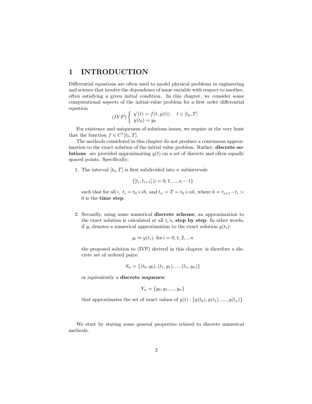
CHAPTER VI NUMERICAL INTEGRATION OF ORDINARY DIFFERENTIAL EQUATIONS Nabil R. Nassif and Dolly K. Fayad December 2012 1 1 INTRODUCTION Differential equations are often used to model physical problems in engineering and science that involve the dependence of some variable with respect to another, often satisfying a given initial condition. In this chapter, we consider some computational aspects of the initial-value problem for a first order differential equation (IV P) � y′(t) = f(t, y(t)) t ∈ [t0, T] y(t0) = y0 For existence and uniqueness of solutions issues, we require at the very least that the function f ∈ C1[t0, T]. The methods considered in this chapter do not produce a continuous approx- imation to the exact solution of the initial value problem. Rather, discrete so- lutions are provided approximating y(t) on a set of discrete and often equally spaced points. Specifically: 1. The interval [t0, T] is first subdivided into n subintervals {[ti, ti+1] |i = 0, 1, ..., n − 1} such that for all i, ti = t0+ih, and tn = T = t0+nh, where h = ti+1−ti > 0 is the time step. 2. Secondly, using some numerical discrete scheme, an approximation to the exact solution is calculated at all ti’s, step by step. In other words, if yi denotes a numerical approximation to the exact solution y(ti): yi ≈ y(ti), for i = 0, 1, 2, ...n the proposed solution to (IVP) derived in this chapter, is therefore a dis- crete set of ordered pairs: Sn = {(t0, y0), (t1, y1), ..., (tn, yn)} or equivalently a discrete sequence: Yn = {y0, y1, ..., yn} that approximates the set of exact values of y(t) : {y(t0), y(t1), ...., y(tn)}. We start by stating some general properties related to discrete numerical methods. 2 • Two types of formulae , explicit or implicit formulae are usually pro- posed for calculating Yn. 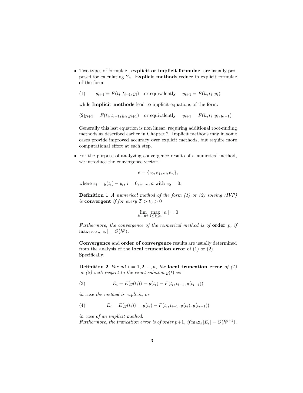Explicit methods reduce to explicit formulae of the form: yi+1 = F(ti, ti+1, yi) or equivalently yi+1 = F(h, ti, yi) (1) while Implicit methods lead to implicit equations of the form: yi+1 = F(ti, ti+1, yi, yi+1) or equivalently yi+1 = F(h, ti, yi, yi+1) (2) Generally this last equation is non linear, requiring additional root-finding methods as described earlier in Chapter 2. Implicit methods may in some cases provide improved accuracy over explicit methods, but require more computational effort at each step. • For the purpose of analyzing convergence results of a numerical method, we introduce the convergence vector: e = {e0, e1, ..., en}, where ei = y(ti) − yi, i = 0, 1, ..., n with e0 = 0. Definition 1 A numerical method of the form (1) or (2) solving (IVP) is convergent if for every T > t0 > 0 lim h→0+ max 1≤i≤n |ei| = 0 Furthermore, the convergence of the numerical method is of order p, if max1≤i≤n |ei| = O(hp). Convergence and order of convergence results are usually determined from the analysis of the local truncation error of (1) or (2). Specifically: Definition 2 For all i = 1, 2, ..., n, the local truncation error of (1) or (2) with respect to the exact solution y(t) is: Ei = E(y(ti)) = y(ti) − F(ti, ti−1, y(ti−1)) (3) in case the method is explicit, or Ei = E(y(ti)) = y(ti) − F(ti, ti−1, y(ti), y(ti−1)) (4) in case of an implicit method. Furthermore, the truncation error is of order p+1, if maxi |Ei| = O(hp+1). 3 Based on the definitions above, the order of convergence of a numerical method is determined as follows: Proposition 1 Let F satisfy the following Lipshitz condition: |F(ti, ti−1, y(ti−1)) − F(ti, ti−1, yi−1)| ≤ K|y(ti) − yi|, (5) If the local truncation error of a numerical method solving (IVP) is O(hp+1), then the convergence of the method is O(hp). Proof. Considering for example, an explicit method whereas from equa- tion (3): y(ti) = F(ti, ti−1, y(ti−1)) + Ei, i = 0, 1, ..., n (6) and since from equation (1): yi = F(ti−1, ti, yi−1) (7) then subtracting (6) and (7) leads to: ei = F(ti, ti−1, y(ti−1)) − F(ti, ti−1, yi−1) + Ei. Thus under the assumption (5), one has: |ei| ≤ K|ei−1| + |Ei|. By induction on the right hand side term (|ei−1|), one has: |ei| ≤ Km|ei−m| + |Ei| + K|Ei−1| + ... + Km−1|Ei−m+1| ; i ≥ m. For m = i with e0 = 0, one obtains: |ei| ≤ |Ei| + K|Ei−1| + ... + Ki−1|E1|; , i ≥ 1. which implies that: |ei| ≤ Σi−1 m=1Ki−1−m|Em|. Since our main interest is in the global behavior of the method, i.e. maxi |ei|, the last inequality indicates that the global error is due to the accumulation of local truncation errors from previous steps. Remark 1 The naive expectation is that since the number of steps n = (T − t0)/h increases as O(h−1), if the truncation error is O(hp+1), then under favorable conditions, the global error would decrease as O(hp). We say then that the method is of order p. 4 In numerical integration of ODE, the Runge-Kutta methods (RK methods) form an important family of implicit and explicit iterative methods for the ap- proximation of solutions of ordinary differential equations (ODE). These tech- niques were developed around 1900 by the German mathematicians C.Runge and M.W.Kutta. In this chapter, we will mainly analyze explicit Runge Kutta schemes that are convergent schemes. The first and simplest RK method for solving the initial-value problem (IVP) considered hereafter is the Explicit-Euler method. 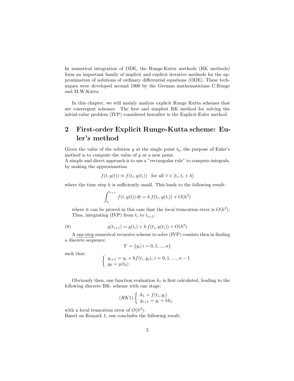2 First-order Explicit Runge-Kutta scheme: Eu- ler’s method Given the value of the solution y at the single point t0, the purpose of Euler’s method is to compute the value of y at a new point. A simple and direct approach is to use a ”rectangular rule” to compute integrals, by making the approximation f(t, y(t)) ≈ f(ti, y(ti)) for all t ∈ [ti, ti + h] where the time step h is sufficiently small. This leads to the following result: � ti+1 ti f(t, y(t)) dt = h f(ti, y(ti)) + O(h2) where it can be proved in this case that the local truncation error is O(h2). Thus, integrating (IVP) from ti to ti+1: y(ti+1) = y(ti) + h f(ti, y(ti)) + O(h2) (8) A one-step numerical recursive scheme to solve (IVP) consists then in finding a discrete sequence: Y = {yi| i = 0, 1, ..., n} such that: � yi+1 = yi + hf(ti, yi), i = 0, 1, ...., n − 1 y0 = y(t0) Obviously then, one function evaluation k1 is first calculated, leading to the following discrete RK- scheme with one stage: (RK1) � k1 = f(ti, yi) yi+1 = yi + hk1 with a local truncation error of O(h2). Based on Remark 1, one concludes the following result: 5 Proposition 2 The Euler’s explicit method is a first order method. (The Global Error of RK1 is O(h)). Example 1 Use Euler’s explicit scheme to solve the following initial value prob- lem with time step h = 0.5: � y′(t) = −1.2y + 7e−0.3t t ∈ [0, 1.5] y(0) = 3 The corresponding discrete scheme with one stage is given by: (RK1) � k1 = −1.2yi + 7e−0.3ti yi+1 = yi + hk1 The numerical results could be presented in a table as follows: i ti yi k1 = −1.2yi + 7e−0.3ti yi+1 = yi + hK1 0 0 y0 = 3 3.4 y1 = 4.7 1 0.5 y1 = 4.7 0.386 y2 = 4.893 2 1 y2 = 4.893 −0.686 y3 = 4.550 3 1.5 y3 = 4.550 × × The discrete set of points solving the given problem is therefore: {(0, 3); (0.5, 4.7); (1, 4.893); (1.5, 4.550); (2, 4.052); (2.5, 3.542)} The analytical or exact solution being y = 70 9 e−0.3t − 43 9 e−1.2t, we can therefore compute the absolute error at each ti value: i ti yi y(ti) E= |y(ti) − yi| 0 0 y0 = 3 y(t0) = 3 E = 0 1 0.5 y1 = 4.7 y(t1) = 4.072 E =−0.6277 2 1 y2 = 4.893 y(t2) = 4.323 E = −0.5696 3 1.5 y3 = 4.550 y(t3) = 4.170 E = 0.3803 3 Second order explicit Runge-Kutta methods The Runge-Kutta methods of order 2 solving the initial value problem (IVP) are ”modified” Euler’ s schemes. 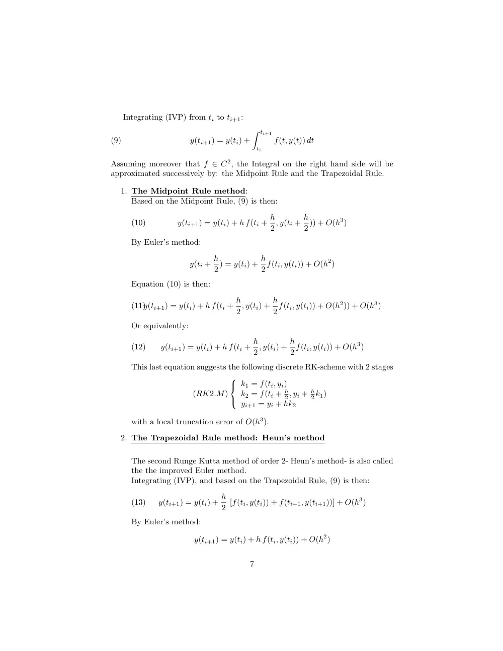The following consequence of the Mean value theorem is needed: Proposition 3 If f : R2 → R is a function of 2 variables and is at least of class C1, then: f(t, y + O(ϵ)) = f(t, y) + O(ϵ) 6 Integrating (IVP) from ti to ti+1: y(ti+1) = y(ti) + � ti+1 ti f(t, y(t)) dt (9) Assuming moreover that f ∈ C2, the Integral on the right hand side will be approximated successively by: the Midpoint Rule and the Trapezoidal Rule. 1. The Midpoint Rule method: Based on the Midpoint Rule, (9) is then: y(ti+1) = y(ti) + h f(ti + h 2 , y(ti + h 2 )) + O(h3) (10) By Euler’s method: y(ti + h 2 ) = y(ti) + h 2 f(ti, y(ti)) + O(h2) Equation (10) is then: y(ti+1) = y(ti) + h f(ti + h 2 , y(ti) + h 2 f(ti, y(ti)) + O(h2)) + O(h3) (11) Or equivalently: y(ti+1) = y(ti) + h f(ti + h 2 , y(ti) + h 2 f(ti, y(ti)) + O(h3) (12) This last equation suggests the following discrete RK-scheme with 2 stages (RK2.M)    k1 = f(ti, yi) k2 = f(ti + h 2 , yi + h 2 k1) yi+1 = yi + hk2 with a local truncation error of O(h3). 2. The Trapezoidal Rule method: Heun’s method The second Runge Kutta method of order 2- Heun’s method- is also called the the improved Euler method. 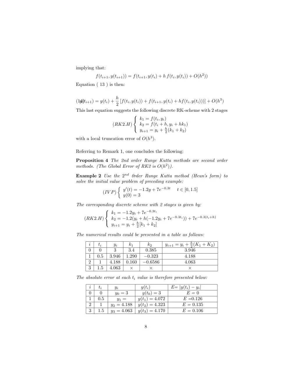Integrating (IVP), and based on the Trapezoidal Rule, (9) is then: y(ti+1) = y(ti) + h 2 [f(ti, y(ti)) + f(ti+1, y(ti+1))] + O(h3) (13) By Euler’s method: y(ti+1) = y(ti) + h f(ti, y(ti)) + O(h2) 7 implying that: f(ti+1, y(ti+1)) = f(ti+1, y(ti) + h f(ti, y(ti)) + O(h2)) Equation ( 13 ) is then: y(ti+1) = y(ti) + h 2 [f(ti, y(ti)) + f(ti+1, y(ti) + hf(ti, y(ti)))] + O(h3) (14) This last equation suggests the following discrete RK-scheme with 2 stages (RK2.H)    k1 = f(ti, yi) k2 = f(ti + h, yi + hk1) yi+1 = yi + h 2 (k1 + k2) with a local truncation error of O(h3). Referring to Remark 1, one concludes the following: Proposition 4 The 2nd order Runge Kutta methods are second order methods. (The Global Error of RK2 is O(h2)). Example 2 Use the 2nd 0rder Runge Kutta method (Heun’s form) to solve the initial value problem of preceding example: (IV P) � y′(t) = −1.2y + 7e−0.3t t ∈ [0, 1.5] y(0) = 3 The corresponding discrete scheme with 2 stages is given by: (RK2.H)    k1 = −1.2yi + 7e−0.3ti k2 = −1.2(yi + h(−1.2yi + 7e−0.3ti)) + 7e−0.3(ti+h) yi+1 = yi + h 2 [k1 + k2] The numerical results could be presented in a table as follows: i ti yi k1 k2 yi+1 = yi + h 2 (K1 + K2) 0 0 3 3.4 0.385 3.946 1 0.5 3.946 1.290 −0.323 4.188 2 1 4.188 0.160 −0.6586 4.063 3 1.5 4.063 × × × The absolute error at each ti value is therefore presented below: i ti yi y(ti) E= |y(ti) − yi| 0 0 y0 = 3 y(t0) = 3 E = 0 1 0.5 y1 = y(t1) = 4.072 E =0.126 2 1 y2 = 4.188 y(t2) = 4.323 E = 0.135 3 1.5 y3 = 4.063 y(t3) = 4.170 E = 0.106 8 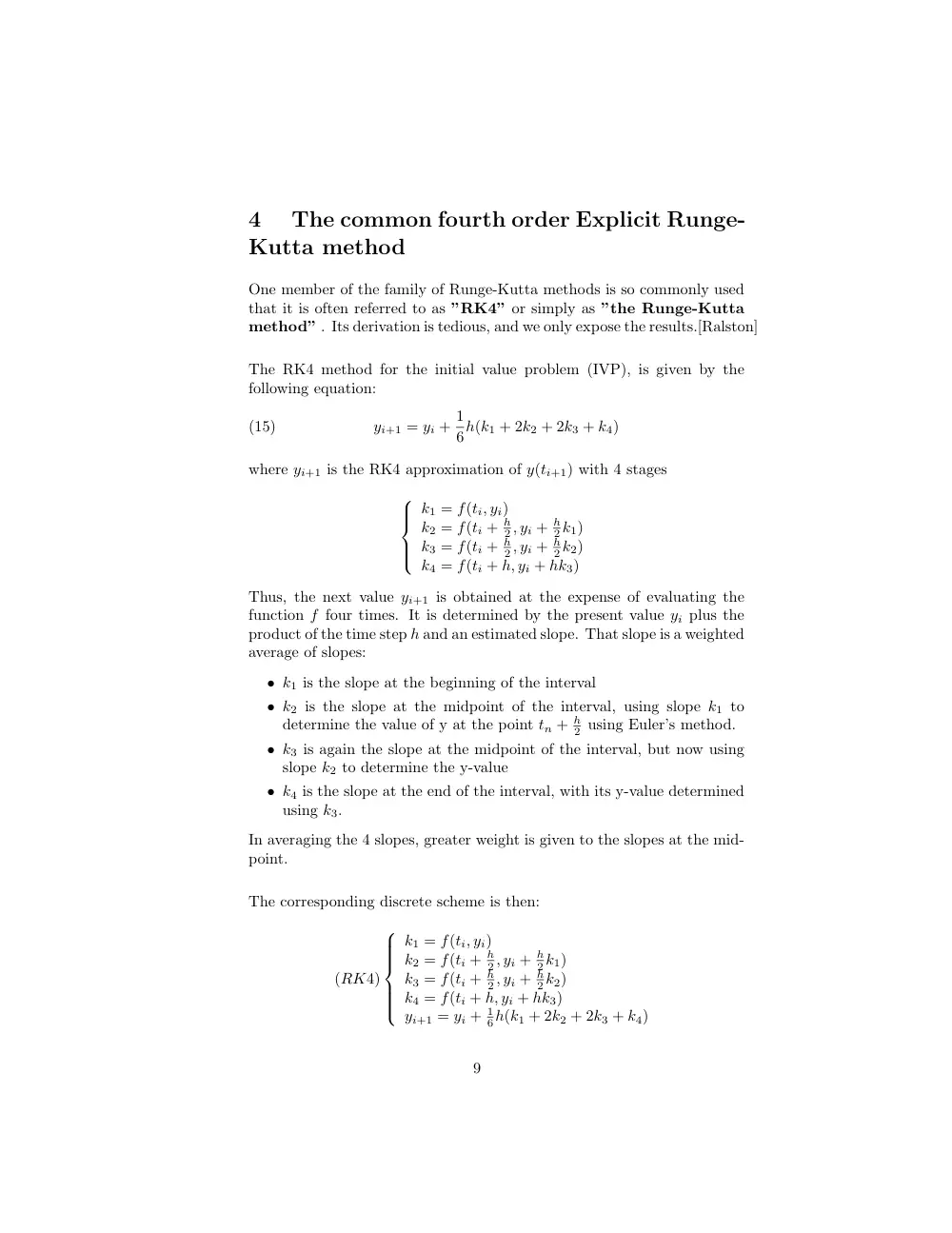4 The common fourth order Explicit Runge- Kutta method One member of the family of Runge-Kutta methods is so commonly used that it is often referred to as ”RK4” or simply as ”the Runge-Kutta method” . Its derivation is tedious, and we only expose the results.[Ralston] The RK4 method for the initial value problem (IVP), is given by the following equation: yi+1 = yi + 1 6h(k1 + 2k2 + 2k3 + k4) (15) where yi+1 is the RK4 approximation of y(ti+1) with 4 stages        k1 = f(ti, yi) k2 = f(ti + h 2 , yi + h 2 k1) k3 = f(ti + h 2 , yi + h 2 k2) k4 = f(ti + h, yi + hk3) Thus, the next value yi+1 is obtained at the expense of evaluating the function f four times. It is determined by the present value yi plus the product of the time step h and an estimated slope. That slope is a weighted average of slopes: • k1 is the slope at the beginning of the interval • k2 is the slope at the midpoint of the interval, using slope k1 to determine the value of y at the point tn + h 2 using Euler’s method. • k3 is again the slope at the midpoint of the interval, but now using slope k2 to determine the y-value • k4 is the slope at the end of the interval, with its y-value determined using k3. In averaging the 4 slopes, greater weight is given to the slopes at the mid- point. The corresponding discrete scheme is then: (RK4)            k1 = f(ti, yi) k2 = f(ti + h 2 , yi + h 2 k1) k3 = f(ti + h 2 , yi + h 2 k2) k4 = f(ti + h, yi + hk3) yi+1 = yi + 1 6h(k1 + 2k2 + 2k3 + k4) 9 Remark 2 As proved in [Butcher] or [Gear], the final formula of the RK4 method agrees with the Taylor series expansion up to the term in h4, meaning that the truncation error per step is O(h5) and that the total accumulated error has order h4. Proposition 5 The RK4 method is a 4th-order method. 10 EXERCISES 1. Use Euler’s method to solve the following (IVP) (a) y′(t) = et−y, 0 ≤ t ≤ 1, y(0) = 1, h = 0.5 (b) y′(t) = −y + ty1/2, 2 ≤ t ≤ 3, y(2) = 2, h = 0.25 (c) y′(t) = 1 + y/t, 1 ≤ t ≤ 2, y(1) = 2, h = 0.25 2. Consider the following Initial Value Problem: (IV P) � dy dt = t2 + y ; t ∈ [1, 2] y(1) = 1 (a) Write first the discrete scheme of Euler’s method, (RK1), then use 2 steps of this scheme to approximate y(1.25) and y(1.50). • Discrete Scheme (RK1) � ................................................................ yi+1 = .................................................... • Express all the computed results with a precision p = 3. i ti yi K1 yi+1 0 . . . . 1 . . . . (b) Write first the discrete scheme of Heun’s method, (RK2.H), then use 2 steps of this scheme to approximate y(1.25) and y(1.50). • Discrete Scheme (RK2.H)    ............................................................... ................................................................ yi+1 = .................................................... • Express all the computed results with a precision p = 3. i ti yi K1 K2 yi+1 0 . . . . . 1 . . . . . 11 (c) Write first the discrete scheme of the Midpoint Rule method, (RK2.M), then use 2 steps of this scheme to approximate y(1.25) and y(1.50). • Discrete Scheme (RK2.M)    ............................................................... ................................................................ yi+1 = .................................................... • Express all the computed results with a precision p = 3. i ti yi K1 K2 yi+1 0 . . . . . 1 . . . . . 3. Use Heun’s method (RK2.H) to solve the following (IVP) 1. y′(t) = te3t − 2y, 0 ≤ t ≤ 1, y(0) = 0, h = 0.5 2. y′(t) = 1 + (t − y)2, 2 ≤ t ≤ 3, y(2) = 1, h = 0.5 3. y′(t) = 1 + y/t, 1 ≤ t ≤ 2, y(1) = 2, h = 0.25 Exercise 4: Repeat Exercise 2 using the Midpoint method (RK2.M) 12