CMPS 251 Homework Assignment 5, Fall 2015

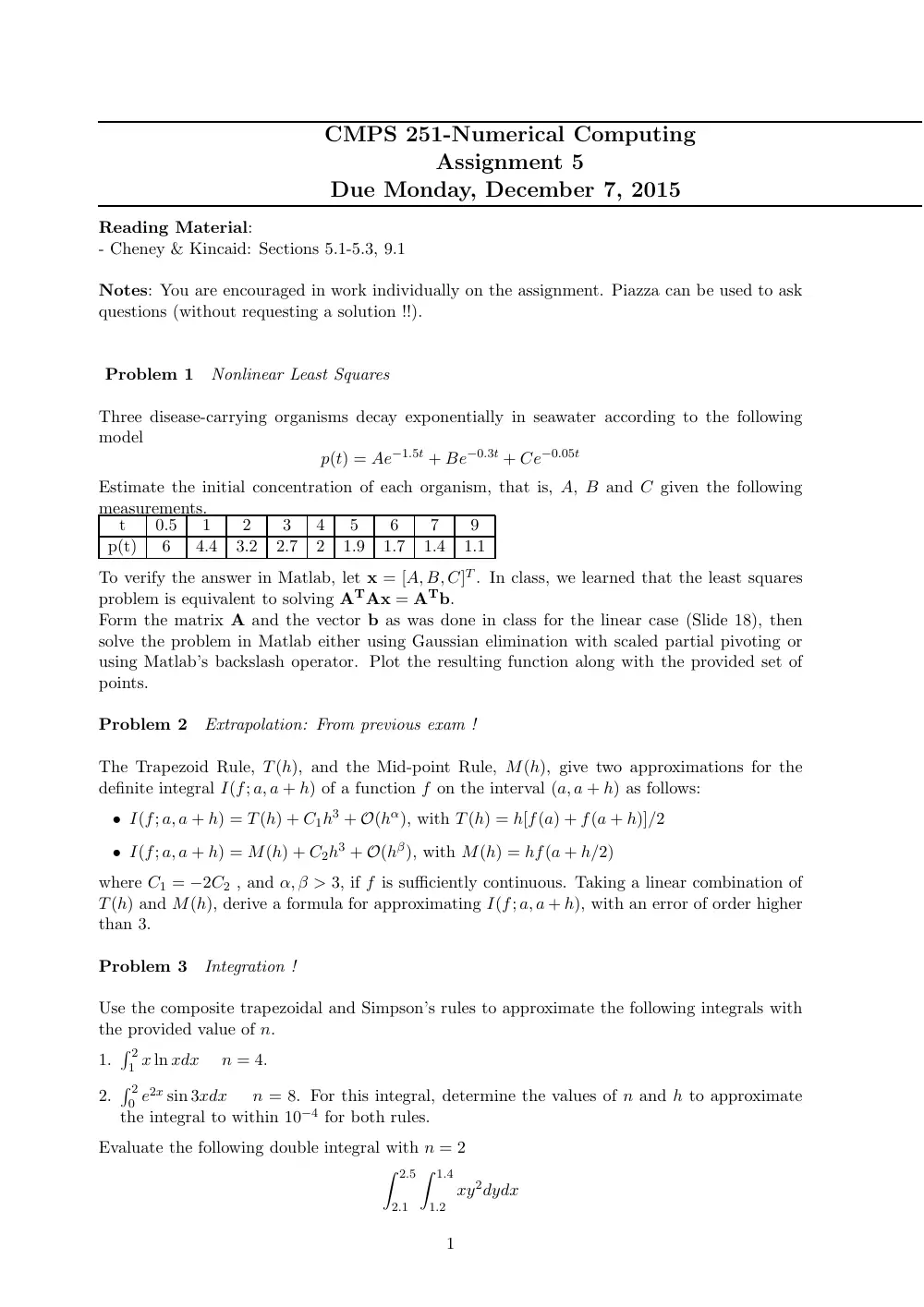
CMPS 251-Numerical Computing Assignment 5 Due Monday, December 7, 2015 Reading Material: - Cheney & Kincaid: Sections 5.1-5.3, 9.1 Notes: You are encouraged in work individually on the assignment. Piazza can be used to ask questions (without requesting a solution !!). Problem 1 Nonlinear Least Squares Three disease-carrying organisms decay exponentially in seawater according to the following model p(t) = Ae−1.5t + Be−0.3t + Ce−0.05t Estimate the initial concentration of each organism, that is, A, B and C given the following measurements. t 0.5 1 2 3 4 5 6 7 9 p(t) 6 4.4 3.2 2.7 2 1.9 1.7 1.4 1.1 To verify the answer in Matlab, let x = [A, B, C]T . In class, we learned that the least squares problem is equivalent to solving ATAx = ATb. Form the matrix A and the vector b as was done in class for the linear case (Slide 18), then solve the problem in Matlab either using Gaussian elimination with scaled partial pivoting or using Matlab’s backslash operator. Plot the resulting function along with the provided set of points. Problem 2 Extrapolation: From previous exam ! The Trapezoid Rule, T(h), and the Mid-point Rule, M(h), give two approximations for the definite integral I(f; a, a + h) of a function f on the interval (a, a + h) as follows: • I(f; a, a + h) = T(h) + C1h3 + O(hα), with T(h) = h[f(a) + f(a + h)]/2 • I(f; a, a + h) = M(h) + C2h3 + O(hβ), with M(h) = hf(a + h/2) where C1 = −2C2 , and α, β > 3, if f is sufficiently continuous. Taking a linear combination of T(h) and M(h), derive a formula for approximating I(f; a, a + h), with an error of order higher than 3. Problem 3 Integration ! Use the composite trapezoidal and Simpson’s rules to approximate the following integrals with the provided value of n. 1. � 2 1 x ln xdx n = 4. 2. � 2 0 e2x sin 3xdx n = 8. For this integral, determine the values of n and h to approximate the integral to within 10−4 for both rules. 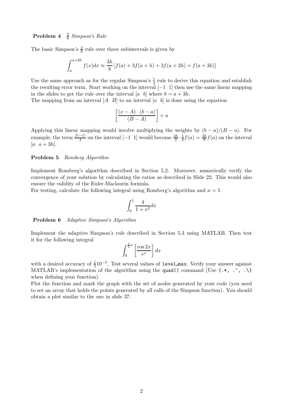Evaluate the following double integral with n = 2 � 2.5 2.1 � 1.4 1.2 xy2dydx 1 Problem 4 3 8 Simpson’s Rule The basic Simpson’s 3 8 rule over three subintervals is given by � a+3h a f(x)dx ≈ 3h 8 [f(a) + 3f(a + h) + 3f(a + 2h) + f(a + 3h)] Use the same approach as for the regular Simpson’s 1 3 rule to derive this equation and establish the resulting error term. Start working on the interval [−1 1] then use the same linear mapping in the slides to get the rule over the interval [a b] where b = a + 3h. The mapping from an interval [A B] to an interval [a b] is done using the equation �(x − A) · (b − a) (B − A) � + a Applying this linear mapping would involve multiplying the weights by (b − a)/(B − a). For example, the term f(−1) 4 on the interval [−1 1] would become 3h 2 · 1 4f(a) = 3h 8 f(a) on the interval [a a + 3h]. Problem 5 Romberg Algorithm Implement Romberg’s algorithm described in Section 5.2. Moreover, numerically verify the convergence of your solution by calculating the ratios as described in Slide 22. This would also ensure the validity of the Euler-Maclaurin formula. For testing, calculate the following integral using Romberg’s algorithm and n = 5 � 1 0 4 1 + x2 dx Problem 6 Adaptive Simpson’s Algorithm Implement the adaptive Simpson’s rule described in Section 5.3 using MATLAB. Then test it for the following integral � 5 4π 0 �cos 2x ex � dx with a desired accuracy of 1 210−3. Test several values of level max. Verify your answer against MATLAB’s implementation of the algorithm using the quad() command (Use {.*, .^, .\} when defining your function). Plot the function and mark the graph with the set of nodes generated by your code (you need to set an array that holds the points generated by all calls of the Simpson function). You should obtain a plot similar to the one in slide 37. 2