CMPS 251 Homework Assignment 6, Fall 2015

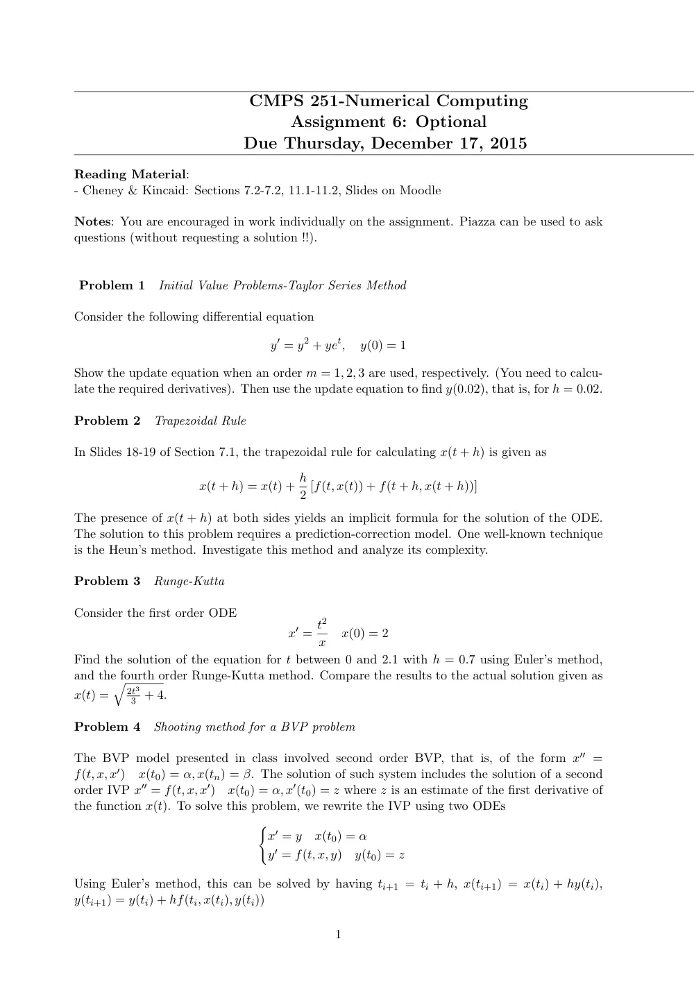
CMPS 251-Numerical Computing Assignment 6: Optional Due Thursday, December 17, 2015 Reading Material: - Cheney & Kincaid: Sections 7.2-7.2, 11.1-11.2, Slides on Moodle Notes: You are encouraged in work individually on the assignment. Piazza can be used to ask questions (without requesting a solution !!). Problem 1 Initial Value Problems-Taylor Series Method Consider the following differential equation y′ = y2 + yet, y(0) = 1 Show the update equation when an order m = 1, 2, 3 are used, respectively. (You need to calcu- late the required derivatives). Then use the update equation to find y(0.02), that is, for h = 0.02. Problem 2 Trapezoidal Rule In Slides 18-19 of Section 7.1, the trapezoidal rule for calculating x(t + h) is given as x(t + h) = x(t) + h 2 [f(t, x(t)) + f(t + h, x(t + h))] The presence of x(t + h) at both sides yields an implicit formula for the solution of the ODE. The solution to this problem requires a prediction-correction model. One well-known technique is the Heun’s method. Investigate this method and analyze its complexity. Problem 3 Runge-Kutta Consider the first order ODE x′ = t2 x x(0) = 2 Find the solution of the equation for t between 0 and 2.1 with h = 0.7 using Euler’s method, and the fourth order Runge-Kutta method. Compare the results to the actual solution given as x(t) = √ 2t3 3 + 4. Problem 4 Shooting method for a BVP problem The BVP model presented in class involved second order BVP, that is, of the form x′′ = f(t, x, x′) x(t0) = α, x(tn) = β. The solution of such system includes the solution of a second order IVP x′′ = f(t, x, x′) x(t0) = α, x′(t0) = z where z is an estimate of the first derivative of the function x(t). 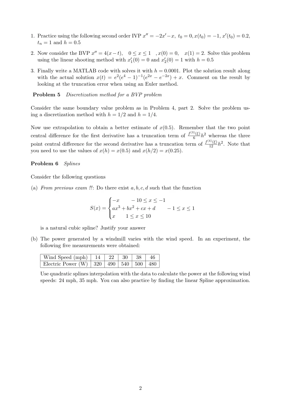To solve this problem, we rewrite the IVP using two ODEs { x′ = y x(t0) = α y′ = f(t, x, y) y(t0) = z Using Euler’s method, this can be solved by having ti+1 = ti + h, x(ti+1) = x(ti) + hy(ti), y(ti+1) = y(ti) + hf(ti, x(ti), y(ti)) 1 1. Practice using the following second order IVP x′′ = −2x′−x, t0 = 0, x(t0) = −1, x′(t0) = 0.2, tn = 1 and h = 0.5 2. Now consider the BVP x′′ = 4(x − t), 0 ≤ x ≤ 1 , x(0) = 0, x(1) = 2. Solve this problem using the linear shooting method with x′ 1(0) = 0 and x′ 2(0) = 1 with h = 0.5 3. Finally write a MATLAB code with solves it with h = 0.0001. Plot the solution result along with the actual solution x(t) = e2(e4 − 1)−1(e2x − e−2x) + x. Comment on the result by looking at the truncation error when using an Euler method. Problem 5 Discretization method for a BVP problem Consider the same boundary value problem as in Problem 4, part 2. Solve the problem us- ing a discretization method with h = 1/2 and h = 1/4. Now use extrapolation to obtain a better estimate of x(0.5). Remember that the two point central difference for the first derivative has a truncation term of f(3)(ξ) 6 h2 whereas the three point central difference for the second derivative has a truncation term of f(4)(ξ) 12 h2. Note that you need to use the values of x(h) = x(0.5) and x(h/2) = x(0.25). Problem 6 Splines Consider the following questions (a) From previous exam !!: Do there exist a, b, c, d such that the function S(x) =      −x − 10 ≤ x ≤ −1 ax3 + bx2 + cx + d − 1 ≤ x ≤ 1 x 1 ≤ x ≤ 10 is a natural cubic spline? Justify your answer (b) The power generated by a windmill varies with the wind speed. In an experiment, the following five measurements were obtained: Wind Speed (mph) 14 22 30 38 46 Electric Power (W) 320 490 540 500 480 Use quadratic splines interpolation with the data to calculate the power at the following wind speeds: 24 mph, 35 mph. You can also practice by finding the linear Spline approximation. 2