EECE 380 Problems Solution Manual, Fall 2011

25 Chapter 2: Transmission Lines Lesson #4 Chapter — Section: 2-1, 2-2 Topics: Lumped-element model Highlights: • TEM lines • General properties of transmission lines • L, C, R, G 26 Lesson #5 Chapter — Section: 2-3, 2-4 Topics: Transmission-line equations, wave propagation Highlights: • Wave equation • Characteristic impedance • General solution Special Illustrations: • Example 2-1 27 Lesson #6 Chapter — Section: 2-5 Topics: Lossless line Highlights: • General wave propagation properties • Reflection coefficient • Standing waves • Maxima and minima Special Illustrations: • Example 2-2 • Example 2-5 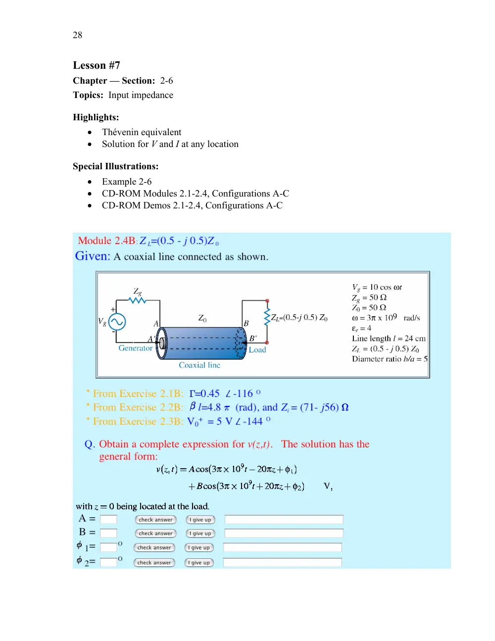28 Lesson #7 Chapter — Section: 2-6 Topics: Input impedance Highlights: • Thévenin equivalent • Solution for V and I at any location Special Illustrations: • Example 2-6 • CD-ROM Modules 2.1-2.4, Configurations A-C • CD-ROM Demos 2.1-2.4, Configurations A-C 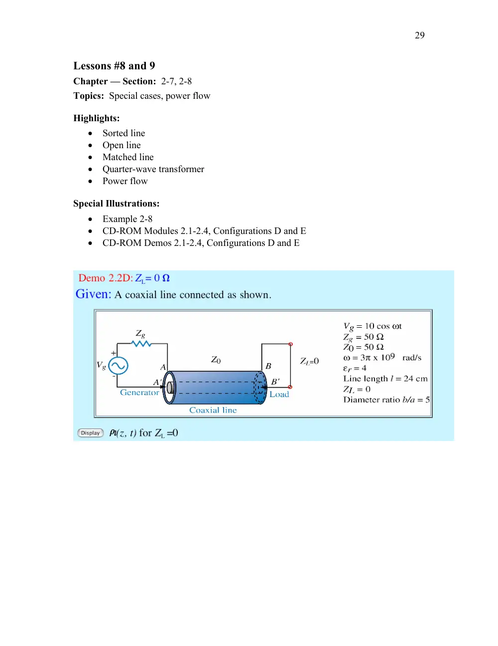29 Lessons #8 and 9 Chapter — Section: 2-7, 2-8 Topics: Special cases, power flow Highlights: • Sorted line • Open line • Matched line • Quarter-wave transformer • Power flow Special Illustrations: • Example 2-8 • CD-ROM Modules 2.1-2.4, Configurations D and E • CD-ROM Demos 2.1-2.4, Configurations D and E 30 Lessons #10 and 11 Chapter — Section: 2-9 Topics: Smith chart Highlights: • Structure of Smith chart • Calculating impedances, admittances, transformations • Locations of maxima and minima Special Illustrations: • Example 2-10 • Example 2-11 31 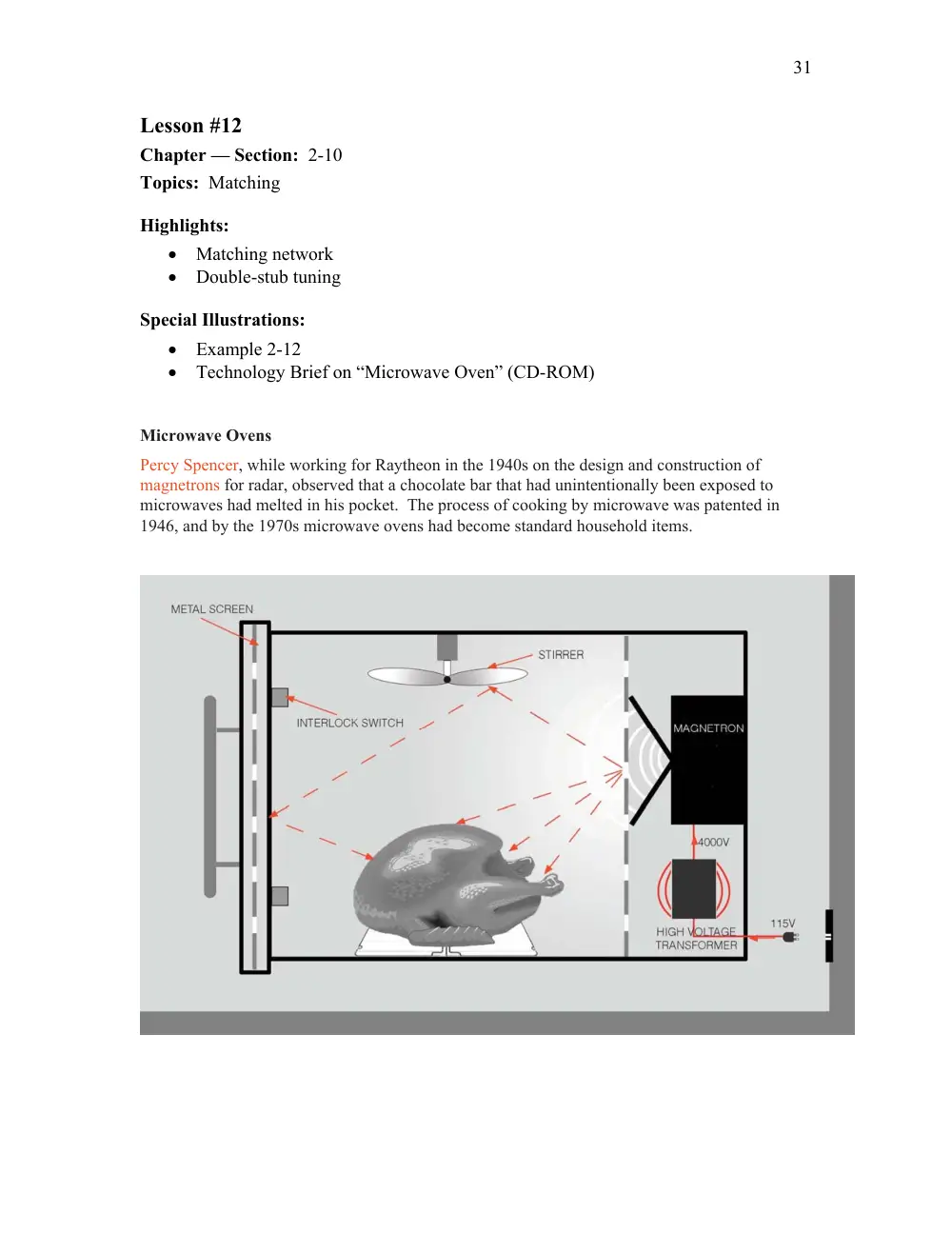Lesson #12 Chapter — Section: 2-10 Topics: Matching Highlights: • Matching network • Double-stub tuning Special Illustrations: • Example 2-12 • Technology Brief on “Microwave Oven” (CD-ROM) Microwave Ovens Percy Spencer, while working for Raytheon in the 1940s on the design and construction of magnetrons for radar, observed that a chocolate bar that had unintentionally been exposed to microwaves had melted in his pocket. The process of cooking by microwave was patented in 1946, and by the 1970s microwave ovens had become standard household items. 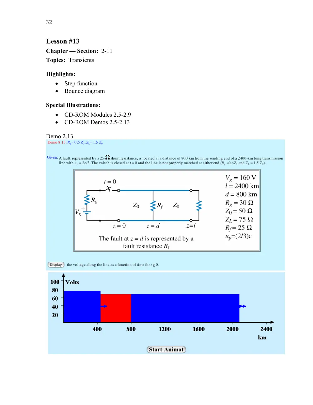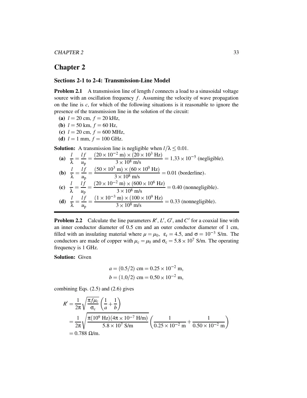32 Lesson #13 Chapter — Section: 2-11 Topics: Transients Highlights: • Step function • Bounce diagram Special Illustrations: • CD-ROM Modules 2.5-2.9 • CD-ROM Demos 2.5-2.13 Demo 2.13 CHAPTER 2 33 Chapter 2 Sections 2-1 to 2-4: Transmission-Line Model Problem 2.1 A transmission line of length l connects a load to a sinusoidal voltage source with an oscillation frequency f. Assuming the velocity of wave propagation on the line is c, for which of the following situations is it reasonable to ignore the presence of the transmission line in the solution of the circuit: (a) l � 20 cm, f � 20 kHz, (b) l � 50 km, f � 60 Hz, (c) l � 20 cm, f � 600 MHz, (d) l � 1 mm, f � 100 GHz. Solution: A transmission line is negligible when l λ � 0 01. (a) l λ � l f up � � 20 10  2 m �� � 20 103 Hz � 3 108 m/s � 1 33 10  5 (negligible). (b) l λ � l f up � � 50 103 m �� � 60 100 Hz � 3 108 m/s � 0 01 (borderline) (c) l λ � l f up � � 20 10  2 m �� � 600 106 Hz � 3 108 m/s � 0 40 (nonnegligible) (d) l λ � l f up � � 1 10  3 m �� � 100 109 Hz � 3 108 m/s � 0 33 (nonnegligible) Problem 2.2 Calculate the line parameters R � , L � , G � , and C � for a coaxial line with an inner conductor diameter of 0 5 cm and an outer conductor diameter of 1 cm, filled with an insulating material where µ � µ0, εr � 4 5, and σ � 10  3 S/m. The conductors are made of copper with µc � µ0 and σc � 5 8 107 S/m. The operating frequency is 1 GHz. Solution: Given a � � 0 5 2 � cm � 0 25 10  2 m � b � � 1 0 2 � cm � 0 50 10  2 m � combining Eqs. (2.5) and (2.6) gives R � � 1 2π � π fµc σc � 1 a � 1 b � 1 2π π � 109 Hz � � 4π 10  7 H/m � 5 8 107 S/m � 1 0 25 10  2 m � 1 0 50 10  2 m � 0 788 Ω/m 34 CHAPTER 2 From Eq. (2.7), L � � µ 2π ln � b a � 4π 10  7 H/m 2π ln2 � 139 nH/m From Eq. (2.8), G � � 2πσ ln � b a � � 2π 10  3 S/m ln2 � 9 1 mS/m From Eq. (2.9), C � � 2πε ln � b a � � 2πεrε0 ln � b a � � 2π 4 5 � 8 854 10  12 F/m � ln2 � 362 pF/m Problem 2.3 A 1-GHz parallel-plate transmission line consists of 1.2-cm-wide copper strips separated by a 0.15-cm-thick layer of polystyrene. Appendix B gives µc � µ0 � 4π 10  7 (H/m) and σc � 5 8 107 (S/m) for copper, and εr � 2 6 for polystyrene. Use Table 2-1 to determine the line parameters of the transmission line. Assume µ � µ0 and σ � 0 for polystyrene. 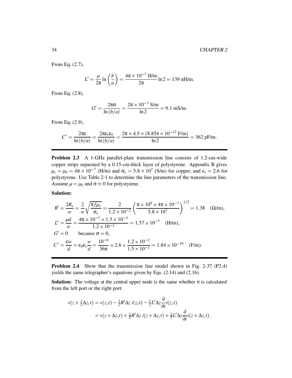Solution: R � � 2Rs w � 2 w � π fµc σc � 2 1 2 10  2 � π 109 4π 10  7 5 8 107 1 � 2 � 1 38 (Ω/m) � L � � µd w � 4π 10  7 1 5 10  3 1 2 10  2 � 1 57 10  7 (H/m) � G � � 0 because σ � 0 � C � � εw d � ε0εr w d � 10  9 36π 2 6 1 2 10  2 1 5 10  3 � 1 84 10  10 (F/m) Problem 2.4 Show that the transmission line model shown in Fig. 2-37 (P2.4) yields the same telegrapher’s equations given by Eqs. (2.14) and (2.16). Solution: The voltage at the central upper node is the same whether it is calculated from the left port or the right port: v � z � 1 2∆z � t �� v � z � t � � 1 2R � ∆z i � z � t � � 1 2L � ∆z ∂ ∂t i � z � t � � v � z � ∆z � t � � 1 2R � ∆z i � z � ∆z � t � � 1 2L � ∆z ∂ ∂t i � z � ∆z � t � CHAPTER 2 35 G'∆z C'∆z ∆z R'∆z 2 L'∆z 2 R'∆z 2 L'∆z 2 i(z, t) + - + - i(z+∆z, t) v(z, t) v(z+∆z, t) Figure P2.4: Transmission line model. Recognizing that the current through the G � � C � branch is i � z � t � � i � z � ∆z � t � (from Kirchhoff’s current law), we can conclude that i � z � t � � i � z � ∆z � t �� G � ∆z v � z � 1 2∆z � t � � C � ∆z ∂ ∂t v � z � 1 2∆z � t � From both of these equations, the proof is completed by following the steps outlined in the text, ie. rearranging terms, dividing by ∆z, and taking the limit as ∆z � 0. Problem 2.5 Find α � β � up, and Z0 for the coaxial line of Problem 2.2. Solution: From Eq. (2.22), γ � � � R � � jωL � � � G � � jωC � � � � � 0 788 Ω/m � � j � 2π 109 s  1 � � 139 10  9 H/m � � � 9 1 10  3 S/m � � j � 2π 109 s  1 � � 362 10  12 F/m � � � 109 10  3 � j44 5 � m  1 Thus, from Eqs. (2.25a) and (2.25b), α � 0 109 Np/m and β � 44 5 rad/m. From Eq. (2.29), Z0 � R � � jωL � G � � jωC � � � 0 788 Ω/m � � j � 2π 109 s  1 � � 139 10  9 H/m � � 9 1 10  3 S/m � � j � 2π 109 s  1 � � 362 10  12 F/m � � � 19 6 � j0 030 � Ω From Eq. (2.33), up � ω β � 2π 109 44 5 � 1 41 108 m/s 36 CHAPTER 2 Section 2-5: The Lossless Line Problem 2.6 In addition to not dissipating power, a lossless line has two important features: (1) it is dispertionless (µp is independent of frequency) and (2) its characteristic impedance Z0 is purely real. Sometimes, it is not possible to design a transmission line such that R �� ωL � and G �� ωC � , but it is possible to choose the dimensions of the line and its material properties so as to satisfy the condition R � C � � L � G � (distortionless line) Such a line is called a distortionless line because despite the fact that it is not lossless, it does nonetheless possess the previously mentioned features of the loss line. Show that for a distortionless line, α � R � � C � L � � � R � G � � β � ω � L � C � � Z0 � � L � C � Solution: Using the distortionless condition in Eq. (2.22) gives γ � α � jβ � � � R � � jωL � � � G � � jωC � � � � L � C � � R � L � � jω � G � C � � jω � � L � C � � R � L � � jω � R � L � � jω � � L � C � � R � L � � jω � R � � C � L � � jω � L � C � Hence, α � �� � γ �� R � � C � L � � β � �� � γ �� ω � L � C � � up � ω β � 1 � L � C � Similarly, using the distortionless condition in Eq. (2.29) gives Z0 � R � � jωL � G � � jωC � � � L � C � R � L � � jω G � C � � jω � � L � C � Problem 2.7 For a distortionless line with Z0 � 50 Ω, α � 20 (mNp/m), up � 2 5 108 (m/s), find the line parameters and λ at 100 MHz. CHAPTER 2 37 Solution: The product of the expressions for α and Z0 given in Problem 2.6 gives R � � αZ0 � 20 10  3 50 � 1 (Ω/m) � and taking the ratio of the expression for Z0 to that for up � ω β � 1 � L � C � gives L � � Z0 up � 50 2 5 108 � 2 10  7 (H/m) � 200 (nH/m) With L � known, we use the expression for Z0 to find C � : C � � L � Z2 0 � 2 10  7 � 50 � 2 � 8 10  11 (F/m) � 80 (pF/m) The distortionless condition given in Problem 2.6 is then used to find G � . G � � R � C � L � � 1 80 10  12 2 10  7 � 4 10  4 (S/m) � 400 (µS/m) � and the wavelength is obtained by applying the relation λ � µp f � 2 5 108 100 106 � 2 5 m Problem 2.8 Find α and Z0 of a distortionless line whose R � � 2 Ω/m and G � � 2 10  4 S/m. Solution: From the equations given in Problem 2.6, α � � R � G � � � 2 2 10  4 � 1 � 2 � 2 10  2 (Np/m) � Z0 � � L � C � � � R � G � � � 2 2 10  4 1 � 2 � 100 Ω Problem 2.9 A transmission line operating at 125 MHz has Z0 � 40 Ω, α � 0 02 (Np/m), and β � 0 75 rad/m. Find the line parameters R � , L � , G � , and C � . Solution: Given an arbitrary transmission line, f � 125 MHz, Z0 � 40 Ω, α � 0 02 Np/m, and β � 0 75 rad/m. Since Z0 is real and α � � 0, the line is distortionless. From Problem 2.6, β � ω � L � C � and Z0 � � L � C � , therefore, L � � βZ0 ω � 0 75 40 2π 125 106 � 38 2 nH/m 38 CHAPTER 2 Then, from Z0 � � L � C � , C � � L � Z2 0 � 38 2 nH/m 402 � 23 9 pF/m From α � � R � G � and R � C � � L � G � , R � � � R � G � � R � G � � � R � G � � L � C � � αZ0 � 0 02 Np/m 40 Ω � 0 6 Ω/m and G � � α2 R � � � 0 02 Np/m � 2 0 8 Ω/m � 0 5 mS/m Problem 2.10 Using a slotted line, the voltage on a lossless transmission line was found to have a maximum magnitude of 1.5 V and a minimum magnitude of 0.6 V. Find the magnitude of the load’s reflection coefficient. Solution: From the definition of the Standing Wave Ratio given by Eq. (2.59), S � � � V � max � � V � min � 1 5 0 6 � 2 5 Solving for the magnitude of the reflection coefficient in terms of S, as in Example 2-4, � Γ � � S � 1 S � 1 � 2 5 � 1 2 5 � 1 � 0 43 Problem 2.11 Polyethylene with εr � 2 25 is used as the insulating material in a lossless coaxial line with characteristic impedance of 50 Ω. The radius of the inner conductor is 1.2 mm. (a) What is the radius of the outer conductor? (b) What is the phase velocity of the line? Solution: Given a lossless coaxial line, Z0 � 50 Ω, εr � 2 25, a � 1 2 mm: (a) From Table 2-2, Z0 � � 60 � εr � ln � b a � which can be rearranged to give b � aeZ0 � εr � 60 � � 1 2 mm � e50 � 2 � 25 � 60 � 4 2 mm CHAPTER 2 39 (b) Also from Table 2-2, up � c � εr � 3 108 m/s � 2 25 � 2 0 108 m/s Problem 2.12 A 50-Ω lossless transmission line is terminated in a load with impedance ZL � � 30 � j50 � Ω. The wavelength is 8 cm. Find: (a) the reflection coefficient at the load, (b) the standing-wave ratio on the line, (c) the position of the voltage maximum nearest the load, (d) the position of the current maximum nearest the load. Solution: (a) From Eq. (2.49a), Γ � ZL � Z0 ZL � Z0 � � 30 � j50 � � 50 � 30 � j50 � � 50 � 0 57e  j79 � 8 � (b) From Eq. (2.59), S � 1 � � Γ � 1 � � Γ � � 1 � 0 57 1 � 0 57 � 3 65 (c) From Eq. (2.56) lmax � θrλ 4π � nλ 2 � � 79 8 � 8 cm 4π π rad 180 � � n 8 cm 2 � � 0 89 cm � 4 0 cm � 3 11 cm (d) A current maximum occurs at a voltage minimum, and from Eq. (2.58), lmin � lmax � λ 4 � 3 11 cm � 8 cm 4 � 1 11 cm Problem 2.13 On a 150-Ω lossless transmission line, the following observations were noted: distance of first voltage minimum from the load � 3 cm; distance of first voltage maximum from the load � 9 cm; S � 3. Find ZL. Solution: Distance between a minimum and an adjacent maximum � λ 4. Hence, 9 cm � 3 cm � 6 cm � λ 4 � 40 CHAPTER 2 or λ � 24 cm. Accordingly, the first voltage minimum is at � min � 3 cm � λ 8. Application of Eq. (2.57) with n � 0 gives θr � 2 2π λ λ 8 � � π � which gives θr � � π 2. � Γ � � S � 1 S � 1 � 3 � 1 3 � 1 � 2 4 � 0 5 Hence, Γ � 0 5e  jπ � 2 � � j0 5. Finally, ZL � Z0 � 1 � Γ 1 � Γ � � 150 � 1 � j0 5 1 � j0 5 � � � 90 � j120 � Ω Problem 2.14 Using a slotted line, the following results were obtained: distance of first minimum from the load � 4 cm; distance of second minimum from the load � 14 cm, voltage standing-wave ratio � 1 5. If the line is lossless and Z0 � 50 Ω, find the load impedance. Solution: Following Example 2.5: Given a lossless line with Z0 � 50 Ω, S � 1 5, lmin � 0 � � 4 cm, lmin � 1 � � 14 cm. Then lmin � 1 � � lmin � 0 � � λ 2 or λ � 2 � lmin � 1 � � lmin � 0 � �� 20 cm and β � 2π λ � 2π rad/cycle 20 cm/cycle � 10π rad/m From this we obtain θr � 2βlmin � n � � � 2n � 1 � π rad � 2 10π rad/m 0 04 m � π rad � � 0 2π rad � � 36 0 � Also, � Γ � � S � 1 S � 1 � 1 5 � 1 1 5 � 1 � 0 2 CHAPTER 2 41 So ZL � Z0 � 1 � Γ 1 � Γ � 50 � 1 � 0 2e  j36 � 0 � 1 � 0 2e  j36 � 0 �� � � 67 0 � j16 4 � Ω Problem 2.15 A load with impedance ZL � � 25 � j50 � Ω is to be connected to a lossless transmission line with characteristic impedance Z0, with Z0 chosen such that the standing-wave ratio is the smallest possible. What should Z0 be? Solution: Since S is monotonic with � Γ � (i.e., a plot of S vs. � Γ � is always increasing), the value of Z0 which gives the minimum possible S also gives the minimum possible � Γ � , and, for that matter, the minimum possible � Γ � 2. A necessary condition for a minimum is that its derivative be equal to zero: 0 � ∂ ∂Z0 � Γ � 2 � ∂ ∂Z0 � RL � jXL � Z0 � 2 � RL � jXL � Z0 � 2 � ∂ ∂Z0 � RL � Z0 � 2 � X2 L � RL � Z0 � 2 � X2 L � 4RL � Z2 0 � � R2 L � X2 L � � � � RL � Z0 � 2 � X2 L � 2 Therefore, Z2 0 � R2 L � X2 L or Z0 � � ZL � � � � 252 � � � 50 � 2 �� 55 9 Ω A mathematically precise solution will also demonstrate that this point is a minimum (by calculating the second derivative, for example). Since the endpoints of the range may be local minima or maxima without the derivative being zero there, the endpoints (namely Z0 � 0 Ω and Z0 � ∞ Ω) should be checked also. Problem 2.16 A 50-Ω lossless line terminated in a purely resistive load has a voltage standing wave ratio of 3. Find all possible values of ZL. Solution: � Γ � � S � 1 S � 1 � 3 � 1 3 � 1 � 0 5 For a purely resistive load, θr � 0 or π. For θr � 0, ZL � Z0 � 1 � Γ 1 � Γ � � 50 � 1 � 0 5 1 � 0 5 � � 150 Ω For θr � π, Γ � � 0 5 and ZL � 50 � 1 � 0 5 1 � 0 5 � � 15 Ω 42 CHAPTER 2 Section 2-6: Input Impedance Problem 2.17 At an operating frequency of 300 MHz, a lossless 50-Ω air-spaced transmission line 2.5 m in length is terminated with an impedance ZL � � 40 � j20 � Ω. Find the input impedance. Solution: Given a lossless transmission line, Z0 � 50 Ω, f � 300 MHz, l � 2 5 m, and ZL � � 40 � j20 � Ω. Since the line is air filled, up � c and therefore, from Eq. (2.38), β � ω up � 2π 300 106 3 108 � 2π rad/m Since the line is lossless, Eq. (2.69) is valid: Zin � Z0 � ZL � jZ0 tanβl Z0 � jZLtanβl � 50 � � 40 � j20 � � j50tan � 2π rad/m 2 5 m � 50 � j � 40 � j20 � tan � 2π rad/m 2 5 m � � 50 � � 40 � j20 � � j50 0 50 � j � 40 � j20 � 0 � � 40 � j20 � Ω Problem 2.18 A lossless transmission line of electrical length l � 0 35λ is terminated in a load impedance as shown in Fig. 2-38 (P2.18). Find Γ, S, and Zin. Zin Z0 = 100 Ω ZL = (60 + j30) Ω l = 0.35λ Figure P2.18: Loaded transmission line. Solution: From Eq. (2.49a), Γ � ZL � Z0 ZL � Z0 � � 60 � j30 � � 100 � 60 � j30 � � 100 � 0 307e j132 � 5 � From Eq. (2.59), S � 1 � � Γ � 1 � � Γ � � 1 � 0 307 1 � 0 307 � 1 89 CHAPTER 2 43 From Eq. (2.63) Zin � Z0 � ZL � jZ0tanβl Z0 � jZLtanβl � 100 � � 60 � j30 � � j100tan � 2π rad λ 0 35λ � 100 � j � 60 � j30 � tan � 2π rad λ 0 35λ � � � � 64 8 � j38 3 � Ω Problem 2.19 Show that the input impedance of a quarter-wavelength long lossless line terminated in a short circuit appears as an open circuit. Solution: Zin � Z0 � ZL � jZ0tanβl Z0 � jZLtanβl For l � λ 4, βl � 2π λ � λ 4 � π 2. With ZL � 0, we have Zin � Z0 � jZ0 tanπ 2 Z0 � j∞ (open circuit) Problem 2.20 Show that at the position where the magnitude of the voltage on the line is a maximum the input impedance is purely real. Solution: From Eq. (2.56), lmax � � θr � 2nπ � 2β, so from Eq. (2.61), using polar representation for Γ, Zin � � lmax �� Z0 � 1 � � Γ � ejθre  j2βlmax 1 � � Γ � ejθre  j2βlmax � � Z0 � 1 � � Γ � ejθre  j � θr � 2nπ � 1 � � Γ � ejθre  j � θr � 2nπ � � � Z0 � 1 � � Γ � 1 � � Γ � � which is real, provided Z0 is real. Problem 2.21 A voltage generator with vg � t � � 5cos � 2π 109t � V and internal impedance Zg � 50 Ω is connected to a 50-Ω lossless air-spaced transmission line. The line length is 5 cm and it is terminated in a load with impedance ZL � � 100 � j100 � Ω. Find (a) Γ at the load. (b) Zin at the input to the transmission line. (c) the input voltage � Vi and input current ˜Ii. 44 CHAPTER 2 Solution: (a) From Eq. (2.49a), Γ � ZL � Z0 ZL � Z0 � � 100 � j100 � � 50 � 100 � j100 � � 50 � 0 62e  j29 � 7 � (b) All formulae for Zin require knowledge of β � ω up. Since the line is an air line, up � c, and from the expression for vg � t � we conclude ω � 2π 109 rad/s. Therefore β � 2π 109 rad/s 3 108 m/s � 20π 3 rad/m Then, using Eq. (2.63), Zin � Z0 � ZL � jZ0 tanβl Z0 � jZLtanβl � 50 � � 100 � j100 � � j50tan � 20π 3 rad/m 5 cm � 50 � j � 100 � j100 � tan � 20π 3 rad/m 5 cm � � � 50 � � 100 � j100 � � j50tan � π 3 rad � 50 � j � 100 � j100 � tan � π 3 rad � � � � 12 5 � j12 7 � Ω An alternative solution to this part involves the solution to part (a) and Eq. (2.61). (c) In phasor domain, � Vg � 5 V ej0 � . From Eq. (2.64), � Vi � � VgZin Zg � Zin � 5 � 12 5 � j12 7 � 50 � � 12 5 � j12 7 � � 1 40e  j34 � 0 � (V) � and also from Eq. (2.64), � Ii � � Vi Zin � 1 4e  j34 � 0 � � 12 5 � j12 7 � � 78 4ej11 � 5 � (mA) Problem 2.22 A 6-m section of 150-Ω lossless line is driven by a source with vg � t �� 5cos � 8π 107t � 30 � � (V) and Zg � 150 Ω. If the line, which has a relative permittivity εr � 2 25, is terminated in a load ZL � � 150 � j50 � Ω � find (a) λ on the line, (b) the reflection coefficient at the load, (c) the input impedance, CHAPTER 2 45 (d) the input voltage � Vi, (e) the time-domain input voltage vi � t � . Solution: vg � t �� 5cos � 8π 107t � 30 � � V � � Vg � 5e  j30 � V Vg Ii Zg Zin Z0 ZL ~ Vi~ ~ + + - + - - VL ~ IL ~ + - Transmission line Generator Load z = -l z = 0 Vg Ii Zg Zin ~ Vi~ ~ + - ⇓ 150 Ω (150-j50) Ω l = 6 m = 150 Ω Figure P2.22: Circuit for Problem 2.22. (a) up � c � εr � 3 108 � 2 25 � 2 108 (m/s) � λ � up f � 2πup ω � 2π 2 108 8π 107 � 5 m � β � ω up � 8π 107 2 108 � 0 4π (rad/m) � βl � 0 4π 6 � 2 4π (rad) 46 CHAPTER 2 Since this exceeds 2π (rad), we can subtract 2π, which leaves a remainder βl � 0 4π (rad). (b) Γ � ZL � Z0 ZL � Z0 � 150 � j50 � 150 150 � j50 � 150 � � j50 300 � j50 � 0 16e  j80 � 54 � . (c) Zin � Z0 � ZL � jZ0tanβl Z0 � jZLtanβl � � 150 � � 150 � j50 � � j150tan � 0 4π � 150 � j � 150 � j50 � tan � 0 4π � � � � 115 70 � j27 42 � Ω (d) � Vi � � VgZin Zg � Zin � 5e  j30 � � 115 7 � j27 42 � 150 � 115 7 � j27 42 � 5e  j30 � � 115 7 � j27 42 265 7 � j27 42 � 5e  j30 � 0 44ej7 � 44 � � 2 2e  j22 � 56 � (V) (e) vi � t �� �� � � Viejωt � � �� � 2 2e  j22 � 56 � ejωt � � 2 2cos � 8π 107t � 22 56 � � V Problem 2.23 Two half-wave dipole antennas, each with impedance of 75 Ω, are connected in parallel through a pair of transmission lines, and the combination is connected to a feed transmission line, as shown in Fig. 2.39 (P2.23(a)). All lines are 50 Ω and lossless. (a) Calculate Zin1, the input impedance of the antenna-terminated line, at the parallel juncture. (b) Combine Zin1 and Zin2 in parallel to obtain Z �L, the effective load impedance of the feedline. (c) Calculate Zin of the feedline. Solution: (a) Zin1 � Z0 � ZL1 � jZ0tanβl1 Z0 � jZL1 tanβl1 � � 50 � 75 � j50tan � � 2π λ � � 0 2λ �� 50 � j75tan � � 2π λ � � 0 2λ ��� � � 35 20 � j8 62 � Ω CHAPTER 2 47 0.2λ 0.2λ 75 Ω (Antenna) 75 Ω (Antenna) Zin 0.3λ Zin Zin 1 2 Figure P2.23: (a) Circuit for Problem 2.23. (b) Z �L � Zin1Zin2 Zin1 � Zin2 � � 35 20 � j8 62 � 2 2 � 35 20 � j8 62 � � � 17 60 � j4 31 � Ω (c) Zin l = 0.3λ ZL' Figure P2.23: (b) Equivalent circuit. Zin � 50 � � 17 60 � j4 31 � � j50tan � � 2π λ � � 0 3λ �� 50 � j � 17 60 � j4 31 � tan � � 2π λ � � 0 3λ ��� � � 107 57 � j56 7 � Ω 48 CHAPTER 2 Section 2-7: Special Cases Problem 2.24 At an operating frequency of 300 MHz, it is desired to use a section of a lossless 50-Ω transmission line terminated in a short circuit to construct an equivalent load with reactance X � 40 Ω. If the phase velocity of the line is 0 75c, what is the shortest possible line length that would exhibit the desired reactance at its input? Solution: β � ω up � � 2π rad/cycle �� � 300 106 cycle/s � 0 75 � 3 108 m/s � � 8 38 rad/m On a lossless short-circuited transmission line, the input impedance is always purely imaginary; i.e., Zsc in � jXsc in . Solving Eq. (2.68) for the line length, l � 1 β tan  1 � Xsc in Z0 � 1 8 38 rad/m tan  1 � 40 Ω 50 Ω � � 0 675 � nπ � rad 8 38 rad/m � for which the smallest positive solution is 8 05 cm (with n � 0). Problem 2.25 A lossless transmission line is terminated in a short circuit. How long (in wavelengths) should the line be in order for it to appear as an open circuit at its input terminals? Solution: From Eq. (2.68), Zsc in � jZ0 tanβl. If βl � � π 2 � nπ � , then Zsc in � j∞ � Ω � . Hence, l � λ 2π  π 2 � nπ  � λ 4 � nλ 2 This is evident from Figure 2.15(d). Problem 2.26 The input impedance of a 31-cm-long lossless transmission line of unknown characteristic impedance was measured at 1 MHz. With the line terminated in a short circuit, the measurement yielded an input impedance equivalent to an inductor with inductance of 0.064 µH, and when the line was open circuited, the measurement yielded an input impedance equivalent to a capacitor with capacitance of 40 pF. Find Z0 of the line, the phase velocity, and the relative permittivity of the insulating material. Solution: Now ω � 2π f � 6 28 106 rad/s, so Zsc in � jωL � j2π 106 0 064 10  6 � j0 4 Ω CHAPTER 2 49 and Zoc in � 1 jωC � 1 � j2π 106 40 10  12 �� � j4000 Ω. From Eq. (2.74), Z0 � � Zsc inZoc in � � � j0 4 Ω � � � j4000 Ω � � 40 Ω Using Eq. (2.75), up � ω β � ωl tan  1 � � Zsc in Zoc in � 6 28 106 0 31 tan  1  � � � j0 4 � � j4000 � � 1 95 106 � � 0 01 � nπ � m/s � where n � 0 for the plus sign and n � 1 for the minus sign. For n � 0, up � 1 94 108 m/s � 0 65c and εr � � c up � 2 � 1 0 652 � 2 4. For other values of n, up is very slow and εr is unreasonably high. Problem 2.27 A 75-Ω resistive load is preceded by a λ 4 section of a 50-Ω lossless line, which itself is preceded by another λ 4 section of a 100-Ω line. What is the input impedance? Solution: The input impedance of the λ 4 section of line closest to the load is found from Eq. (2.77): Zin � Z2 0 ZL � 502 75 � 33 33 Ω The input impedance of the line section closest to the load can be considered as the load impedance of the next section of the line. By reapplying Eq. (2.77), the next section of λ 4 line is taken into account: Zin � Z2 0 ZL � 1002 33 33 � 300 Ω Problem 2.28 A 100-MHz FM broadcast station uses a 300-Ω transmission line between the transmitter and a tower-mounted half-wave dipole antenna. The antenna impedance is 73 Ω. You are asked to design a quarter-wave transformer to match the antenna to the line. (a) Determine the electrical length and characteristic impedance of the quarter- wave section. (b) If the quarter-wave section is a two-wire line with d � 2 5 cm, and the spacing between the wires is made of polystyrene with εr � 2 6, determine the physical length of the quarter-wave section and the radius of the two wire conductors. 50 CHAPTER 2 Solution: (a) For a match condition, the input impedance of a load must match that of the transmission line attached to the generator. A line of electrical length λ 4 can be used. From Eq. (2.77), the impedance of such a line should be Z0 � � ZinZL � � 300 73 � 148 Ω (b) λ 4 � up 4f � c 4 � εr f � 3 108 4 � 2 6 100 106 � 0 465 m � and, from Table 2-2, Z0 � 120 � ε ln � � d 2a � � d 2a 2 � 1 � Ω Hence, ln � � d 2a � � d 2a 2 � 1 � � 148 � 2 6 120 � 1 99 � which leads to � d 2a � � d 2a 2 � 1 � 7 31 � and whose solution is a � d 7 44 � 25 cm 7 44 � 3 36 mm. Problem 2.29 A 50-MHz generator with Zg � 50 Ω is connected to a load ZL � � 50 � j25 � Ω. The time-average power transferred from the generator into the load is maximum when Zg � Z L � where Z L is the complex conjugate of ZL. To achieve this condition without changing Zg, the effective load impedance can be modified by adding an open-circuited line in series with ZL, as shown in Fig. 2-40 (P2.29). If the line’s Z0 � 100 Ω, determine the shortest length of line (in wavelengths) necessary for satisfying the maximum-power-transfer condition. Solution: Since the real part of ZL is equal to Zg, our task is to find l such that the input impedance of the line is Zin � � j25 Ω, thereby cancelling the imaginary part of ZL (once ZL and the input impedance the line are added in series). Hence, using Eq. (2.73), � j100cotβl � j25 � CHAPTER 2 51 Vg Z L ~ + - (50-j25) Ω Z0 = 100 Ω l 50 Ω Figure P2.29: Transmission-line arrangement for Problem 2.29. or cotβl � � 25 100 � � 0 25 � which leads to βl � � 1 326 or 1 816 Since l cannot be negative, the first solution is discarded. The second solution leads to l � 1 816 β � 1 816 � 2π λ � � 0 29λ Problem 2.30 A 50-Ω lossless line of length l � 0 375λ connects a 300-MHz generator with � Vg � 300 V and Zg � 50 Ω to a load ZL. Determine the time-domain current through the load for: (a) ZL � � 50 � j50 � Ω � (b) ZL � 50 Ω, (c) ZL � 0 (short circuit). Solution: (a) ZL � � 50 � j50 � Ω, βl � 2π λ 0 375λ � 2 36 (rad) � 135 � . Γ � ZL � Z0 ZL � Z0 � 50 � j50 � 50 50 � j50 � 50 � � j50 100 � j50 � 0 45e  j63 � 43 � Application of Eq. (2.63) gives: Zin � Z0 � ZL � jZ0 tanβl Z0 � jZLtanβl � � 50 � � 50 � j50 � � j50tan135 � 50 � j � 50 � j50 � tan135 � � � � 100 � j50 � Ω 52 CHAPTER 2 Vg Zin Z0 ZL ~ + - + - Transmission line Generator Load z = -l z = 0 Vg Ii Zin ~ Vi~ ~ + - ⇓� (50-j50) Ω l = 0.375 λ = 50 Ω 50 Ω Zg Figure P2.30: Circuit for Problem 2.30(a). Using Eq. (2.66) gives V � 0 � � � VgZin Zg � Zin � � 1 ejβl � Γe  jβl � 300 � 100 � j50 � 50 � � 100 � j50 � � 1 ej135 � � 0 45e  j63 � 43 � e  j135 � � 150e  j135 � (V) � � IL � V � 0 Z0 � 1 � Γ �� 150e  j135 � 50 � 1 � 0 45e  j63 � 43 � �� 2 68e  j108 � 44 � (A) � iL � t �� �� � � ILejωt � � �� � 2 68e  j108 � 44 � ej6π � 108t � � 2 68cos � 6π 108t � 108 44 � � (A) CHAPTER 2 53 (b) ZL � 50 Ω � Γ � 0 � Zin � Z0 � 50 Ω � V � 0 � 300 50 50 � 50 � 1 ej135 � � 0 � 150e  j135 � (V) � � IL � V � 0 Z0 � 150 50 e  j135 � � 3e  j135 � (A) � iL � t �� �� � 3e  j135 � ej6π � 108t � � 3cos � 6π 108t � 135 � � (A) (c) ZL � 0 � Γ � � 1 � Zin � Z0 � 0 � jZ0 tan135 � Z0 � 0 � jZ0 tan135 � � � j50 (Ω) � V � 0 � 300 � � j50 � 50 � j50 � 1 ej135 � � e  j135 � � 150e  j135 � (V) � � IL � V 0� Z0 � 1 � Γ � � 150e  j135 � 50 � 1 � 1 � � 6e  j135 � (A) � iL � t �� 6cos � 6π 108t � 135 � � (A) Section 2-8: Power Flow on Lossless Line Problem 2.31 A generator with � Vg � 300 V and Zg � 50 Ω is connected to a load ZL � 75 Ω through a 50-Ω lossless line of length l � 0 15λ. (a) Compute Zin, the input impedance of the line at the generator end. (b) Compute � Ii and � Vi. (c) Compute the time-average power delivered to the line, Pin � 1 2 �� � � Vi � I i � . (d) Compute � VL, � IL, and the time-average power delivered to the load, PL � 1 2 �� � � VL � I L � . How does Pin compare to PL? Explain. (e) Compute the time average power delivered by the generator, Pg, and the time average power dissipated in Zg. Is conservation of power satisfied? Solution: 54 CHAPTER 2 Vg Zin Z0 ~ + - + - Transmission line Generator Load z = -l z = 0 Vg Ii Zg Zin ~ Vi~ ~ + - ⇓� l = 0.15 λ = 50 Ω 50 Ω 75 Ω Figure P2.31: Circuit for Problem 2.31. (a) βl � 2π λ 0 15λ � 54 � � Zin � Z0 � ZL � jZ0 tanβl Z0 � jZLtanβl � � 50 � 75 � j50tan54 � 50 � j75tan54 � � � � 41 25 � j16 35 � Ω (b) � Ii � � Vg Zg � Zin � 300 50 � � 41 25 � j16 35 � � 3 24ej10 � 16 � (A) � � Vi � � IiZin � 3 24ej10 � 16 � � 41 25 � j16 35 � � 143 6e  j11 � 46 � (V) CHAPTER 2 55 (c) Pin � 1 2 �� � � Vi � I i � � 1 2 �� � 143 6e  j11 � 46 � 3 24e  j10 � 16 � � � 143 6 3 24 2 cos � 21 62 � �� 216 (W) (d) Γ � ZL � Z0 ZL � Z0 � 75 � 50 75 � 50 � 0 2 � V � 0 � � Vi � 1 ejβl � Γe  jβl � 143 6e  j11 � 46 � ej54 � � 0 2e  j54 � � 150e  j54 � (V) � � VL � V � 0 � 1 � Γ �� 150e  j54 � � 1 � 0 2 �� 180e  j54 � (V) � � IL � V 0� Z0 � 1 � Γ �� 150e  j54 � 50 � 1 � 0 2 �� 2 4e  j54 � (A) � PL � 1 2 �� � � VL � I L � � 1 2 �� � 180e  j54 � 2 4ej54 � � � 216 (W) PL � Pin, which is as expected because the line is lossless; power input to the line ends up in the load. (e) Power delivered by generator: Pg � 1 2 �� � � Vg � Ii � � 1 2 �� � 300 3 24e j10 � 16 � � � 486cos � 10 16 � �� 478 4 (W) Power dissipated in Zg: PZg � 1 2 �� � � Ii � VZg � � 1 2 �� � � Ii � I i Zg � � 1 2 � � Ii � 2Zg � 1 2 � 3 24 � 2 50 � 262 4 (W) Note 1: Pg � PZg � Pin � 478 4 W. Problem 2.32 If the two-antenna configuration shown in Fig. 2-41 (P2.32) is connected to a generator with � Vg � 250 V and Zg � 50 Ω, how much average power is delivered to each antenna? Solution: Since line 2 is λ 2 in length, the input impedance is the same as ZL1 � 75 Ω. The same is true for line 3. At junction C–D, we now have two 75-Ω impedances in parallel, whose combination is 75 2 � 37 5 Ω. Line 1 is λ 2 long. Hence at A–C, input impedance of line 1 is 37.5 Ω, and � Ii � � Vg Zg � Zin � 250 50 � 37 5 � 2 86 (A) � 56 CHAPTER 2 Zin + - Generator 50 Ω λ/2 λ/2 λ/2 ZL = 75 Ω (Antenna 1) ZL = 75 Ω (Antenna 2) A B D C 250 V Line 1 Line 2 Line 3 1 2 Figure P2.32: Antenna configuration for Problem 2.32. Pin � 1 2 �� � � Ii � V i � � 1 2 �� � � Ii � I i � Z in � � � 2 86 � 2 37 5 2 � 153 37 (W) This is divided eq