MATH 201 Chapter 15 Summary, Fall 2011

Chapter 15: Multiple Integrals Section 1: Definition 1: R is a region in the plane. ( f x y) , is a function of 2 variables which is defined on R (i.e. R is contained in Domain f), Then the double integral of f on R is defined as: ( ) ( ) ( ) ∑ ∫∫ = ∆ → ∆ = n i i i i A R A f x y x y dA x y f 0 1 , lim , , Theorem 1: R is a region in the plane. ( f x y) , is a function of 2 variables which is defined on R Then: ( ) ( ) ( ) ⇒ ∫∫    R x y dA x y f R R R x y f , , nice" boundary " a has is closed and bounded contiuous everywhere on , exist. Theorem 2: Fubini’s Theorem: Suppose R is a closed and bounded region in the plane with nice boundary. Suppose ( f x y) , is a function of 2 variables which is continuous everywhere in the R. 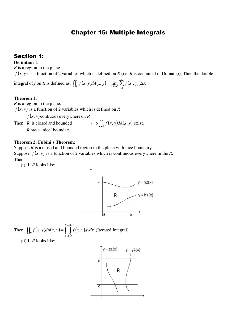Then: (i) If R looks like: Then: ( ) ( ) ( ) ( ) ( ) ∫ ∫ ∫∫ = b a x h x h R f x y dydx x y dA x y f 2 1 , , , (Iterated Integral). 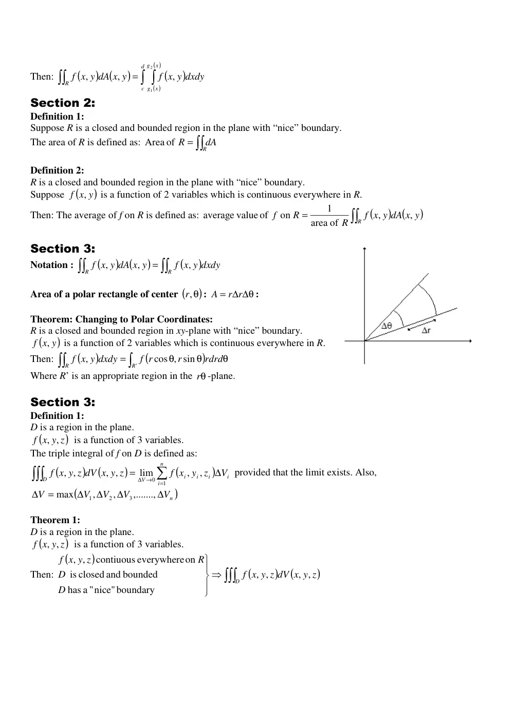(ii) If R looks like: Then: ( ) ( ) ( ) ( ) ( ) ∫ ∫ ∫∫ = d c x g x g R f x y dxdy x y dA x y f 2 1 , , , Section 2: Definition 1: Suppose R is a closed and bounded region in the plane with “nice” boundary. The area of R is defined as: = ∫∫ RdA Area of R Definition 2: R is a closed and bounded region in the plane with “nice” boundary. Suppose ( f x y) , is a function of 2 variables which is continuous everywhere in R. Then: The average of f on R is defined as: ( ) ( ) ∫∫ = R f x y dA x y R R f , , of area 1 average value of on Section 3: Notation : ( ) ( ) ( ) ∫∫ = ∫∫ R R f x y dxdy f x y dA x y , , , Area of a polar rectangle of center ( ,r θ) : = ∆ ∆θ r r A : Theorem: Changing to Polar Coordinates: R is a closed and bounded region in xy-plane with “nice” boundary. ( f x y) , is a function of 2 variables which is continuous everywhere in R. Then: ( ) ( ) ∫ ∫∫ θ θ θ = ' cos , sin , R R rdrd r f r f x y dxdy Where R’ is an appropriate region in the θ r -plane. Section 3: Definition 1: D is a region in the plane. ( )z f x y , , is a function of 3 variables. The triple integral of f on D is defined as: ( ) ( ) ( ) ∑ ∫∫∫ = ∆ → ∆ = n i i i i i V D V y z f x x y z dV x y z f 0 1 , , lim , , , , provided that the limit exists. Also, ( Vn ) V V V V ∆ ∆ ∆ ∆ = ∆ ,......., , , max 3 2 1 Theorem 1: D is a region in the plane. ( f x y z) , , is a function of 3 variables. Then: ( ) ( ) ( ) ⇒ ∫∫∫    D f x y z dV x y z D D R f x y z , , , , nice" boundary " a has is closed and bounded contiuous everywhere on , , Section 5: Definition 1: Suppose D is a closed and bounded region in space with “nice” boundary. Suppose S is a solid which occupies D. Suppose ( )z x y , , δ is the density of D. 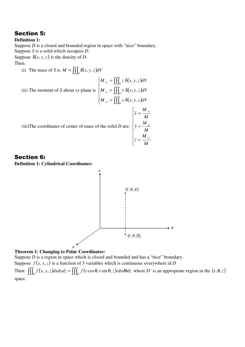Then: (i) The mass of S is ( ) = ∫∫∫ δ D x y z dV M , , (ii) The moment of S about xy-plane is ( ) ( ) ( )       δ = δ = δ = ∫∫∫ ∫∫∫ ∫∫∫ D yz D xz D xy x y z dV x M x y z dV y M x y z dV z M , , , , , , (iii)The coordinates of center of mass of the solid D are:          = = = M M z M M y M M x xy xz yz Section 6: Definition 1: Cylindrical Coordinates: Theorem 1: Changing to Polar Coordinates: Suppose D is a region in space which is closed and bounded and has a “nice” boundary. Suppose ( f x y z) , , is a function of 3 variables which is continuous everywhere id D Then: ( ) ( ) ∫∫∫ ∫∫∫ θ θ θ = ' cos , sin , , , D D z rdrd dz r f r f x y z dxdydz where D’ is an appropriate region in the ( )z r ,θ, space. 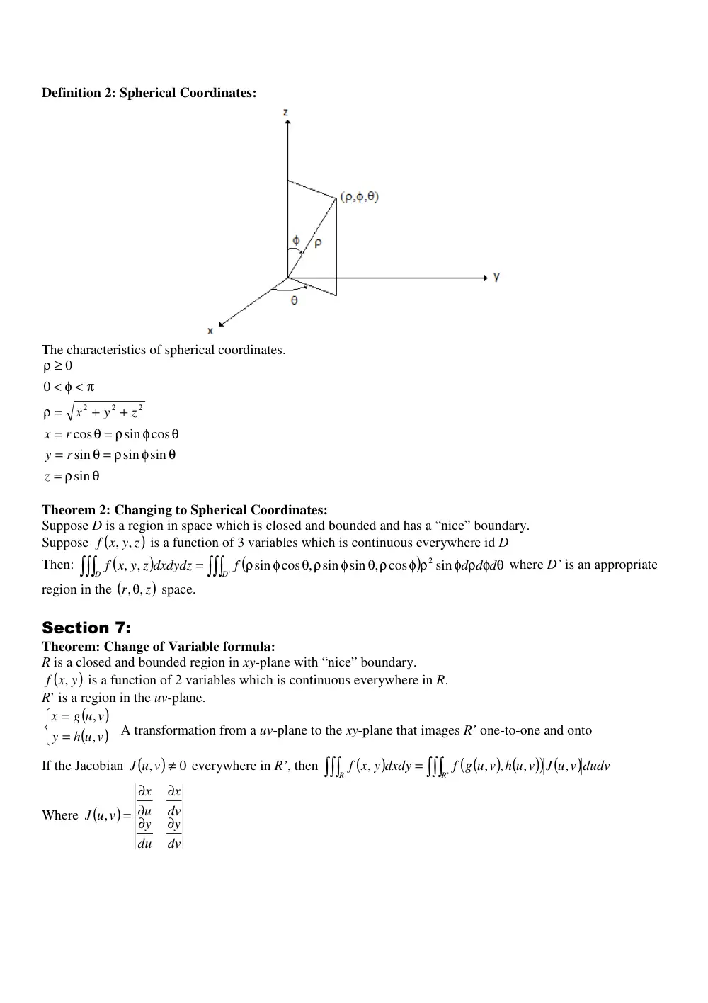Definition 2: Spherical Coordinates: The characteristics of spherical coordinates. θ = ρ θ φ θ = ρ = θ φ θ = ρ = + + = ρ < φ < π ≥ ρ sin sin sin sin sin cos cos 0 0 2 2 2 z r y r x z y x Theorem 2: Changing to Spherical Coordinates: Suppose D is a region in space which is closed and bounded and has a “nice” boundary. Suppose ( f x y z) , , is a function of 3 variables which is continuous everywhere id D Then: ( ) ( ) ∫∫∫ ∫∫∫ φ ρ φ θ φ ρ θ ρ φ θ ρ φ ρ = ' 2 sin sin cos , sin sin , cos , , D D d d d f f x y z dxdydz where D’ is an appropriate region in the ( )z r ,θ, space. Section 7: Theorem: Change of Variable formula: R is a closed and bounded region in xy-plane with “nice” boundary. ( f x y) , is a function of 2 variables which is continuous everywhere in R. R’ is a region in the uv-plane. A transformation from a uv-plane to the xy-plane that images R’ one-to-one and onto If the Jacobian ( ) 0 , J u v ≠ everywhere in R’, then ( ) ( ) ( ) ( ) ( ) ∫∫∫ ∫∫∫ = ' , , , , , R R J u v dudv f g u v h u v f x y dxdy Where ( ) dv y du y dv x u x J u v ∂ ∂ ∂ ∂ ∂ = , ( ) ( )    = = h u v y g u v x , ,