MATH 201 Chapter 16 Summary, Fall 2011

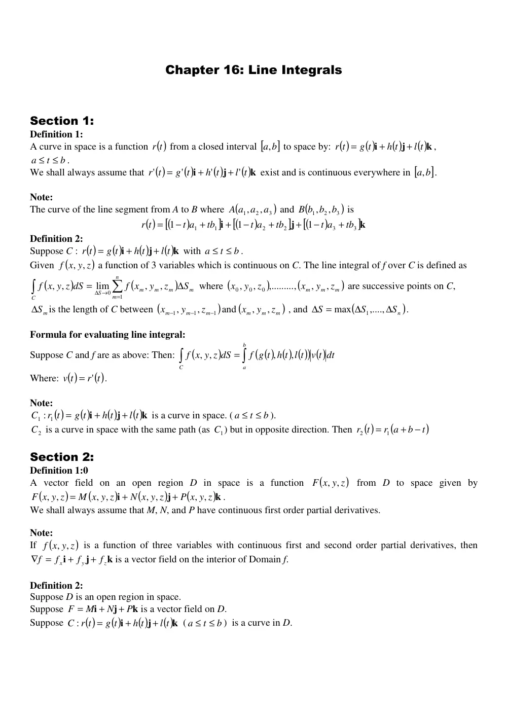
Chapter 16: Line Integrals Section 1: Definition 1: A curve in space is a function ( )t r from a closed interval [ a,b] to space by: ( ) ( ) ( ) ( )k j i l t h t g t r t + + = , b t a ≤ ≤ . We shall always assume that ( ) ( ) ( ) ( )k j i l t h t g t r t ' ' ' ' + + = exist and is continuous everywhere in [ a,b] . Note: The curve of the line segment from A to B where ( 3 ) 2 1 , , a A a a and ( 3 ) 2 1 , , B b b b is ( ) ( ) [ ] ( ) [ ] ( ) [ ]k j i 3 3 2 2 1 1 1 1 1 tb t a tb t a tb t a r t + − + + − + + − = Definition 2: Suppose C : ( ) ( ) ( ) ( )k j i l t h t g t r t + + = with b t a ≤ ≤ . Given ( f x y z) , , a function of 3 variables which is continuous on C. The line integral of f over C is defined as ( ) ( ) ∫ ∑ = ∆ → ∆ = C n m m m m m S S z y f x x y z dS f 1 0 , , lim , , where ( ) ( m ) m m z y x z y x , , ,........., , , 0 0 0 are successive points on C, ∆Sm is the length of C between ( ) ( ) , , and , , 1 1 1 m m m m m m z y x z y x − − − , and ( Sn ) S S ∆ ∆ = ∆ ,...., max 1 . Formula for evaluating line integral: Suppose C and f are as above: Then: ( ) ( ( ) ( ) ( ) ) ( ) ∫ ∫ = b a C f g t h t l t v t dt f x y z dS , , , , Where: ( ) r ( )t v t = ' . Note: ( ) ( ) ( ) ( )k j i l t h t g t r t C + + = 1 : 1 is a curve in space. ( b t a ≤ ≤ ). 2 C is a curve in space with the same path (as 1 C ) but in opposite direction. 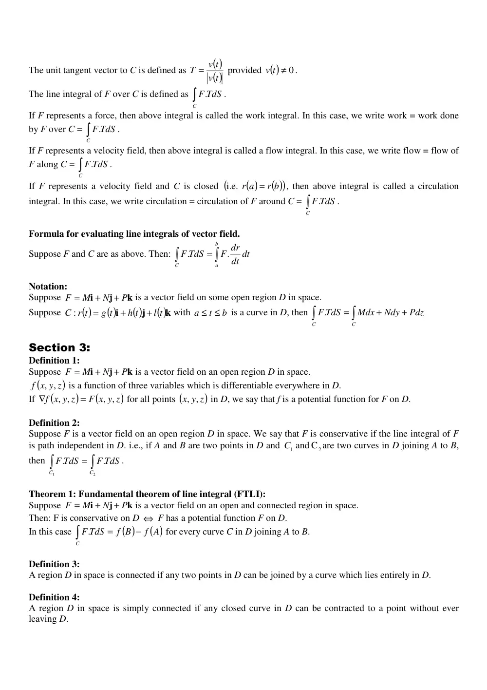Then ( ) ( )t b r a r t − + = 1 2 Section 2: Definition 1:0 A vector field on an open region D in space is a function ( )z F x y , , from D to space given by ( ) ( ) ( ) ( )k j i P x y z N x y z M x y z F x y z , , , , , , , , + + = . We shall always assume that M, N, and P have continuous first order partial derivatives. Note: If ( f x y z) , , is a function of three variables with continuous first and second order partial derivatives, then k j i z y x f f f f + + ∇ = is a vector field on the interior of Domain f. Definition 2: Suppose D is an open region in space. Suppose k j i P N M F + + = is a vector field on D. Suppose ( ) ( ) ( ) ( )k j i l t h t g t C r t + + = : ( b t a ≤ ≤ ) is a curve in D. The unit tangent vector to C is defined as ( ) v( )t T = v t provided ( ) v t ≠ 0 . The line integral of F over C is defined as ∫ C F.TdS . If F represents a force, then above integral is called the work integral. In this case, we write work = work done by F over C = ∫ C F.TdS . If F represents a velocity field, then above integral is called a flow integral. In this case, we write flow = flow of F along C = ∫ C F.TdS . If F represents a velocity field and C is closed ( ) ( ) ( r b ) r a = i.e. , then above integral is called a circulation integral. In this case, we write circulation = circulation of F around C = ∫ C F.TdS . Formula for evaluating line integrals of vector field. Suppose F and C are as above. Then: ∫ ∫ = b a C dt dt F dr F TdS . . Notation: Suppose k j i P N M F + + = is a vector field on some open region D in space. Suppose ( ) ( ) ( ) ( )k j i l t h t g t C r t + + = : with b t a ≤ ≤ is a curve in D, then ∫ ∫ + + = C C Pdz Ndy Mdx F.TdS Section 3: Definition 1: Suppose k j i P N M F + + = is a vector field on an open region D in space. ( )z f x y , , is a function of three variables which is differentiable everywhere in D. If ( ) ( )z F x y f x y z , , , , = ∇ for all points ( )z x y , , in D, we say that f is a potential function for F on D. Definition 2: Suppose F is a vector field on an open region D in space. We say that F is conservative if the line integral of F is path independent in D. i.e., if A and B are two points in D and 2 1 C and C are two curves in D joining A to B, then ∫ ∫ = 2 1 . . C C F TdS F TdS . Theorem 1: Fundamental theorem of line integral (FTLI): Suppose k j i P N M F + + = is a vector field on an open and connected region in space. Then: F is conservative on D ⇔ F has a potential function F on D. In this case ( ) ( ) f A f B TdS F C − = ∫ . for every curve C in D joining A to B. Definition 3: A region D in space is connected if any two points in D can be joined by a curve which lies entirely in D. Definition 4: A region D in space is simply connected if any closed curve in D can be contracted to a point without ever leaving D. 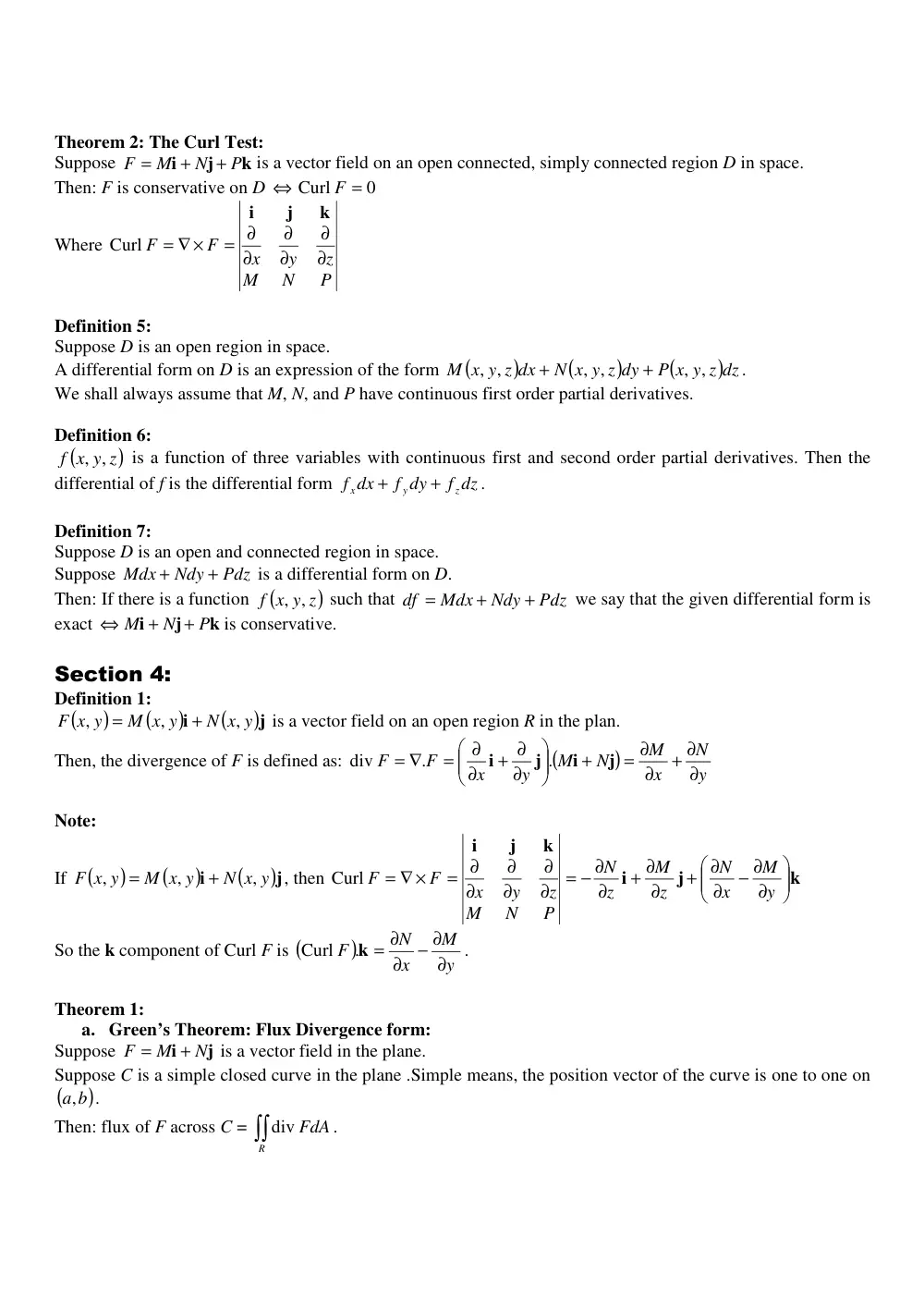Theorem 2: The Curl Test: Suppose k j i P N M F + + = is a vector field on an open connected, simply connected region D in space. Then: F is conservative on D ⇔ 0 Curl F = Where P N M z y x F F ∂ ∂ ∂ ∂ ∂ = ∂ ∇ × = k j i Curl Definition 5: Suppose D is an open region in space. A differential form on D is an expression of the form ( ) ( ) ( P x y z)dz N x y z dy M x y z dx , , , , , , + + . We shall always assume that M, N, and P have continuous first order partial derivatives. Definition 6: ( )z f x y , , is a function of three variables with continuous first and second order partial derivatives. Then the differential of f is the differential form f dz f dy dx f z y x + + . Definition 7: Suppose D is an open and connected region in space. Suppose Pdz Ndy Mdx + + is a differential form on D. Then: If there is a function ( f x y z) , , such that Pdz Ndy Mdx df + + = we say that the given differential form is exact k j i P N M + + ⇔ is conservative. Section 4: Definition 1: ( ) ( ) ( )j i N x y M x y F x y , , , + = is a vector field on an open region R in the plan. Then, the divergence of F is defined as: ( ) y N x M N M y x F F ∂ + ∂ ∂ = ∂ +       ∂ + ∂ ∂ ∂ = = ∇ j i j i . . div Note: If ( ) ( ) ( )j i N x y M x y F x y , , , + = , then k j i k j i       ∂ − ∂ ∂ + ∂ ∂ + ∂ ∂ = − ∂ ∂ ∂ ∂ ∂ ∂ = ∂ = ∇ × y M x N z M z N P N M z y x F Curl F So the k component of Curl F is ( ) y M x N F ∂ − ∂ ∂ = ∂ k. Curl . Theorem 1: a. Green’s Theorem: Flux Divergence form: Suppose j i N M F + = is a vector field in the plane. Suppose C is a simple closed curve in the plane .Simple means, the position vector of the curve is one to one on ( a,b) . Then: flux of F across C = ∫∫ R div FdA . 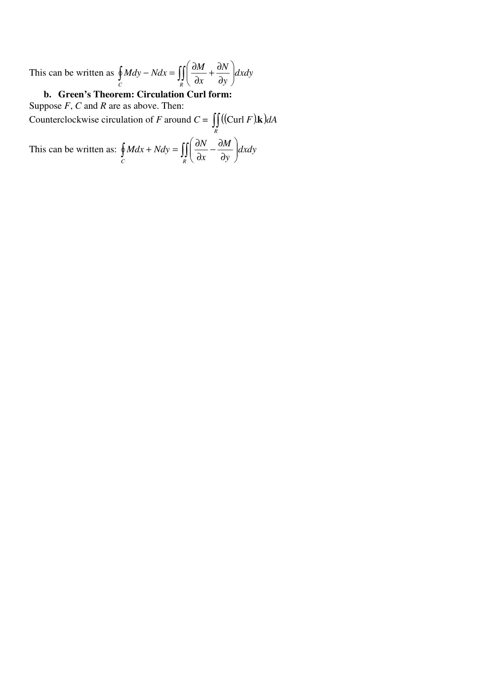This can be written as ∫∫ ∫       ∂ + ∂ ∂ ∂ = − R C y dxdy N x M Ndx Mdy b. Green’s Theorem: Circulation Curl form: Suppose F, C and R are as above. Then: Counterclockwise circulation of F around C = ( ) ( ) ∫∫ R dA Curl F k. This can be written as: ∫∫ ∫       ∂ − ∂ ∂ ∂ = + R C dxdy y M x N Ndy Mdx