MECH 430 Notes 4, Spring 2014

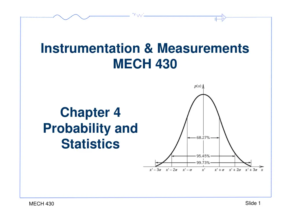
Instrumentation & Measurements MECH 430 MECH 430 Slide 1 Chapter 4 Probability and Statistics 4.1 Introduction • For a given set of measurement, we want to be able to quantify: – A single representative value that best characterize the average of the data set – A representative value that provides a measure of the variation in the measured data set – How well the single average value represents the true average value of the variable MECH 430 Slide 2 4.1 Introduction • In this chapter we will see: – Statistical characteristics of a data set. – Histogram of measured data – Probability density functions to describe the behavior of a variable. – Confidence interval about the measured mean – Perform regression analysis to quantify the confidence interval MECH 430 Sensor characteristics Slide 3 4.2 Statistical Measurement • A sample of data refers to a set of data obtained during repeated measurements of a variable under fixed operating conditions. Systematic errors are considered zero. • The measurement problem will try to estimate the true value of the variable (x’), base on repeated measurement of (x). • The true value is the mean of all possible values of x. 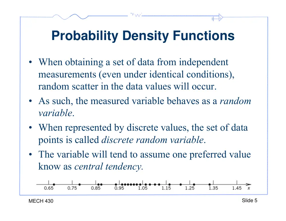MECH 430 Slide 4 Probability Density Functions • When obtaining a set of data from independent measurements (even under identical conditions), random scatter in the data values will occur. • As such, the measured variable behaves as a random variable. • When represented by discrete values, the set of data points is called discrete random variable. • The variable will tend to assume one preferred value know as central tendency. MECH 430 Slide 5 Probability Density Functions • The frequency with which the measured variable assumes a particular value or interval of values is described by its probability density. • The x axis is divided between the maximum and the minimum measured values of x into K intervals. • Let nj be the number of samples that falls in one interval, and 2δx the width of the interval. • For small number of samples, K should be chosen such that nj >5 for at least one interval. 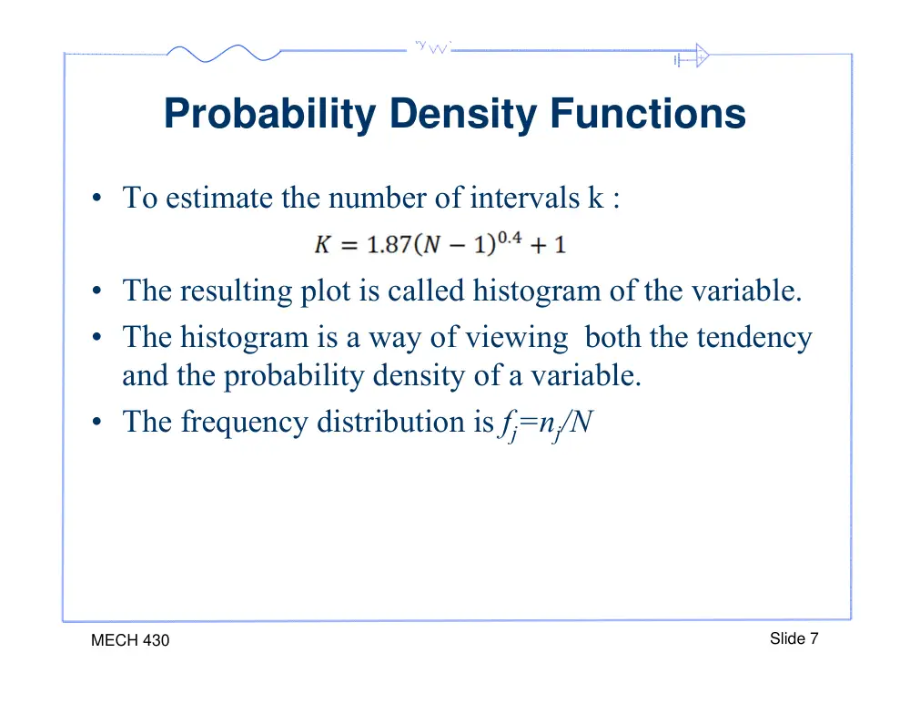MECH 430 Slide 6 Probability Density Functions • To estimate the number of intervals k : • The resulting plot is called histogram of the variable. 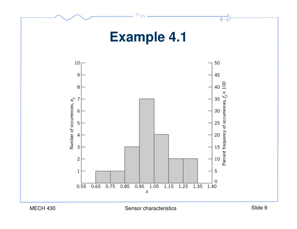• The histogram is a way of viewing both the tendency and the probability density of a variable. 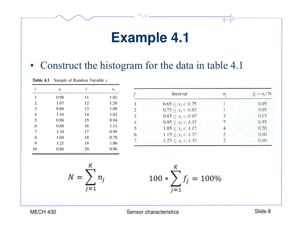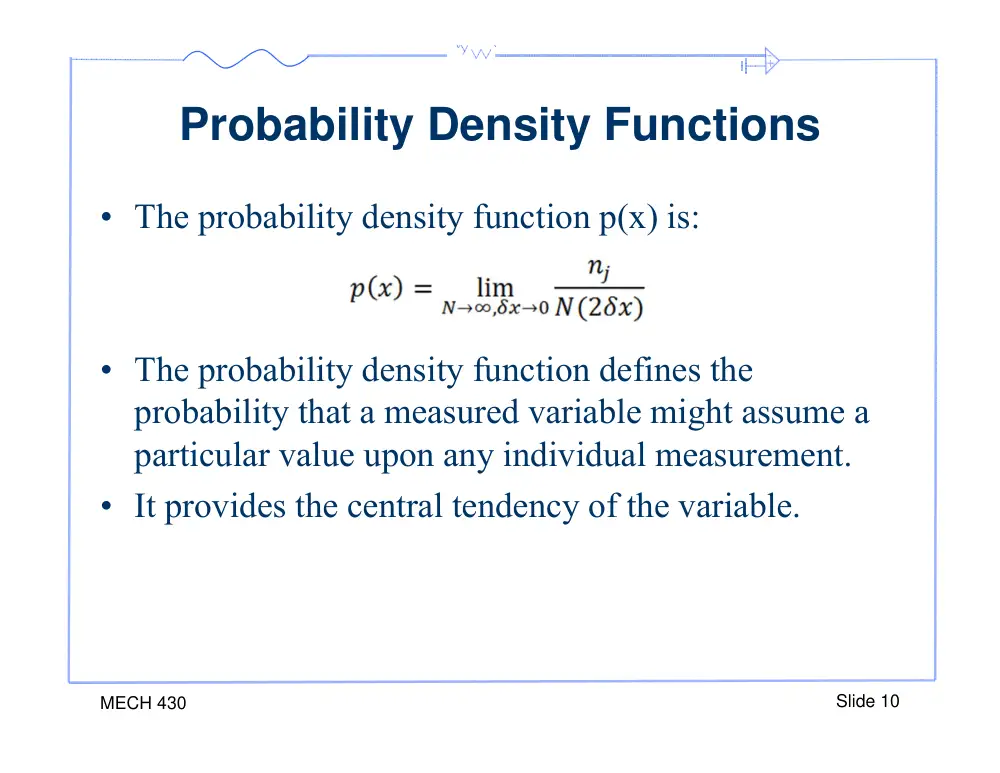• The frequency distribution is fj=nj/N MECH 430 Slide 7 Example 4.1 • Construct the histogram for the data in table 4.1 MECH 430 Sensor characteristics Slide 8 Example 4.1 MECH 430 Sensor characteristics Slide 9 Probability Density Functions • The probability density function p(x) is: • The probability density function defines the probability that a measured variable might assume a particular value upon any individual measurement. • It provides the central tendency of the variable. MECH 430 Slide 10 Probability Density Functions MECH 430 Slide 11 Probability Density Functions • Regardless of the type of distribution assumed by a variable, if the variable shows a central tendency, it can be described and quantified through its mean and variance. • The standard deviation is defined as the square root of the variance. MECH 430 Slide 12 4.3 Infinite Statistics • Many measurands common to engineering are described by a normal or Gaussian distribution where data will scatter symmetrically about some central tendency. • The PDF for a random variable x having a normal distribution is: where x’ is the true mean value and σ2 is the true variance of x MECH 430 Slide 13 4.3 Infinite Statistics • The probability P(x) that the random variable x will assume a value within the interval x’±δx is given by the area under p(x). • Using the following transformation: MECH 430 Slide 14 P(x' x  x  x' x)  p(x)dx x ' x x ' x 4.3 Infinite Statistics • The half value of the probability is tabulated for the interval defined by z1. • The probability that x have a value between x’±z1σ is 2P(z1)x100. MECH 430 Slide 15 MECH 430 Slide 16 Example 4.3 • It is known that the statistics of a voltage signal are given by x’=8.5v and σ2 =2.25V2. If a single measurement of the voltage is made, determine the probability that the measured value is between 10.0 and 11.5V. MECH 430 Slide 17 4.3 Infinite Statistics • Normal or Gaussian. • The PDF for a random variable x having a normal distribution is: MECH 430 Slide 18 P(x' x  x  x' x)  p(x)dx x ' x x ' x 4.3 Infinite Statistics • The probability that x is between x‘±z1σ is 2P(z1)x100. MECH 430 Slide 19 MECH 430 Slide 20 Example • A professor's exam scores are approximately distributed normally with mean 80 and standard deviation 5. • What is the probability that a student scores an 82 or less? Prob(X ≤ 82) = Prob(Z ≤ (82-80)/5) = Prob(Z ≤ .40) = 0.5 + 0.1554 = .6554 • What is the probability that a student scores a 90 or more? Prob(X ≥ 90) = Prob(Z ≥ (90-80)/5) = Prob(Z ≥ 2.00) = 0.5 – 0.4772 = .0228 MECH 430 Slide 21 Example • What is the probability that a student scores a 74 or less? Prob(X ≤ 74) = Prob(Z ≤ (74-80)/5) = Prob(Z ≤ -1.20) • If your table does not have negatives, use: Prob(Z ≤ -1.20) = Prob(Z ≥ 1.20) = 0.5 - .3849 = .1151 MECH 430 Slide 22 Example • What is the probability that a student scores between 78 and 88? Prob(78 ≤ X ≤ 88) = Prob((78-80)/5 ≤ Z ≤ (88- 80)/5) = Prob(-0.40 ≤ Z ≤ 1.60) = Prob(Z ≤ 1.60) -Prob(Z ≤ -0.40) = 0.4452 +0.1554= .6006 4.4 Finite Statistics • If N measurements of x have been made and N is a finite value, the statistical value obtained from such data set will be regarded as estimates of the true values. • Finite sized data sets can provide the statistical estimates know as the sample mean value, the sample variance and the sample standard deviation. MECH 430 Slide 23 4.4 Finite Statistics • While infinite statistics (what we have seen so far) describes the true behavior of a variable, finite statistics describes the behavior of the finite data set. • Here we talk about: – The sample mean, – The sample variance, – The sample standard deviation MECH 430 Slide 24 x  1 N xi i1 N  Sx 2  1 N 1 xi  x  i1 N  2 Sx  1 N 1 xi  x  2 i1 N      1/2 4.4 Finite Statistics • The degrees of freedom in the data set “v” is given as N-1. • The predictive utility of infinite statistics can be extended to data sets for finite sample size with some modification. • For finite sets, the z variable does not provide a reliable weight estimate. • To compensate for the difference, the sample variance is weighted as follows: MECH 430 Slide 25 4.4 Finite Statistics • When sample sizes are small (N < 31 ) the z variable is not accurate. Instead we use the student t distribution. MECH 430 Slide 26 xi  x  tv,PSx (P%) t testimator v is the number of degrees of freedom (N-1) P is the desired probability 4.4 Finite Statistics MECH 430 Slide 27 Example 4.4 • Consider the data in the table below. Compute the sample statistics for this set. Estimate the interval of values over which 95% of the measurements should be expected to lie. MECH 430 Slide 28 • Mean x = 1.02 • Standard deviation Sx = 0.16 • Given the probability 95%, find the corresponding range of data, in other words determined xi • ti = (xi – x)/Sx gives xi = Sx*ti + x • For this example, x19,95 = Sx*t19,95 + x From the Student’s t distribution table, t19,95 = 2.093 thus x19,95 = 0.16*2.093 + 1.02 = 0.33 + 1.02 Interval in which 95% of the data would lie is:1.02 +/- 0.33 MECH 430 Slide 29 Example 4.4 (cont.) Standard Deviation of the Means • Each time we take a new sample we expect a different mean and standard deviation. • The set of mean values will be normally distributed about a central value, even if the PDF of the original function is not itself normal. • The amount of variation in the sample means depends on the sample variance and the size N. MECH 430 Slide 30 Sx  Sx N Standard Deviation of the Means MECH 430 Slide 31 True Mean Value • The standard deviation of the means represents a measure of how well the sample mean represents the true mean. • In the absence of systematic errors in a measurement, the confidence interval states the true value within a likely range about the sample mean value. MECH 430 Slide 32 x'  x  tv,PSx Example 4.4 • Consider the data in the table below. The mean is 1.02 and the standard variation is 0.16. Estimate the true mean value of the measurand at 95% probability based on this finite data set. MECH 430 Slide 33 Example 4.4 • The probability that the true Mean lies between 0.94 and 1.1 is 95%. • Or there are a 95% probability that the true mean will lie between 0.94 and 1.1 (1.02±0.08=1.02±2.93x0.04=1.02±2.93x(0.16/Sqrt(20) MECH 430 Slide 34 Example 4.4 MECH 430 Slide 35 • Mean x = 1.02 • Standard of the means deviation Sx = 0.04 • Given the probability 95%, find the corresponding range of mean values, in other words determined xi • ti = (xi – x)/Sx gives xi = Sx*ti + x • For this example, x19,95 = Sx*t19,95 + x From the Student’s t distribution table, t19,95 = 2.093 thus x19,95 = 0.04*2.093 + 1.02 = 0.08 + 1.02 Interval in which 95% of the means would lie is:1.02 +/- 0.08 MECH 430 Slide 36 Example • A rotary displacement sensor was tested 16 times and recorded in degrees as follows: 0.11, 0.12, 0.09, 0.10, 0.10, 0.14, 0.08, 0.08, 0.13, 0.10, 0.10, 0.12, 0.08, 0.09, 0.11, 0.15. • If we know the standard deviation Sx to be 0.01, what are the odds that true value should fall within 5% of the sample mean? (Note: You can assume a normal distribution and use the appended chart). MECH 430 Slide 37 Example • To solve this problem we assume that readings are normally distributed. The sample mean is computed as: • Then we use the following to determine z0 or tvP :   .0 10625 .0 15 .0 11 ... .0 12 .0 11 16 1       X P X  zoSx N  x'  X  zoSx N      p • Hence .2 125 100 ( .0 10625) 5 16 ( .0 01)    o o z z MECH 430 Slide 38 Example • If we use z0: – interpolate in the z0 table to find the area under the curve to be 0.4832, – the desired area is : 0.4832(2)= 0.9664, – therefore the odds that the mean resolution falls within 5% of the sample mean is 96.64%. • If we use t15, P = 2.125: – interpolate the tv, P Table to get P ≈ 95% MECH 430 Slide 39 MECH 430 Slide 40 4.6 Regression Analysis • Regression signifies expressing a group of data points by a less perfect state. • In linear regression, that less perfect state is a line. • Linear regression can be done via an optimization technique known as least-squares method, which minimizes the sum of errors between the true y coordinate of a point and its estimated y coordinate via the line representing this point (i.e., regression): 2  yi  y  2 i1 n   yi  b  mxi  2 i1 n  x1 y1 x2 y2  xn yn             MECH 430 Slide 41 4.6 Regression Analysis • To minimize this quantity, take its derivative (with respect to m and b) and set it to zero: 2  yi  y  2 i1 n   yi  b  mxi  2 i1 n  0 and 0 2 2       b m Which results: m  n xiyi i1 n   xi i1 n      yi i1 n      n xi 2 i1 n   xi i1 n      2 and b  xi 2 i1 n      yi i1 n       xiyi i1 n      xi i1 n      n xi 2 i1 n   xi i1 n      2 Example - Calibration • Given: – The voltmeter calibration data: MECH 430 Slide 42 • Plot this data and calibrate. • Determine the static sensitivity at: • X = 5.0 • X = 10.0 • X = 20.0 • For which values is the system more sensitive? Analyze X [cm] Y [V] 0.5 0.4 1.0 1.0 2.0 2.3 5.0 6.9 10.0 15.8 20.0 36.4 50.0 110.1 100.0 253.2 Solution MECH 430 Slide 43 • Using Excel: X [cm] Y [V] 0.5 0.4 1.0 1.0 2.0 2.3 5.0 6.9 10.0 15.8 20.0 36.4 50.0 110.1 100.0 253.2 y = 2.5279x - 6.3009 -50 0 50 100 150 200 250 300 0 50 100 150 Voltage [V] X [cm] Solution MECH 430 Slide 44 • Finding the sensitivity at different points: • X = 5.0, S = 1.8 • X = 10.0, S = 2.1 • X = 20.0, S = 2.5 • As X increases the sensor becomes more sensitive. Non-linear Calibration Curves MECH 430 Slide 45 •If the relationship is nonlinear we can set up a look-up table from the calibration curve. x y