MECH 430 Notes 6, Spring 2014

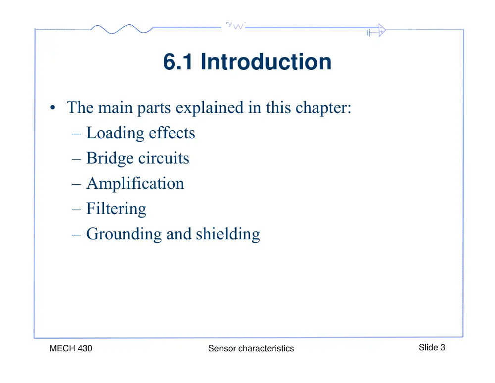
Instrumentation & Measurements MECH 430 MECH 430 Slide 1 Chapter 6 Signal Conditioning 6.1 Introduction MECH 430 Sensor characteristics Slide 2 Physical phenomenon Sensor (Transducer) Signal conditioning Data acquisition PC -Temperature -Pressure -Displacement -Force -Light -Noise -etc.. -Resistive -Inductive -Capacitive -Light -Magnetic -Thermal -Ultrasonic etc.. -Amplification -Linearization -Excitation -Isolation -Averaging -Filtering -Modulation etc.. -Analog multiplexer -Instrumentation amplifier -A/D, D/A conversion -Sample clock -Trigger -Analysis -Feedback control -Display 6.1 Introduction • The main parts explained in this chapter: – Loading effects – Bridge circuits – Amplification – Filtering – Grounding and shielding MECH 430 Sensor characteristics Slide 3 6.3 Loading Error and Impedance Matching MECH 430 Sensor characteristics Slide 4 MECH 430 Sensor characteristics Slide 5 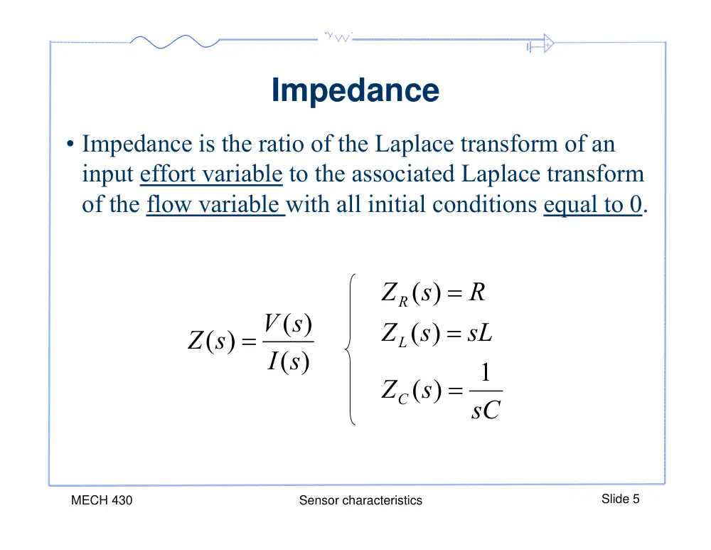Impedance • Impedance is the ratio of the Laplace transform of an input effort variable to the associated Laplace transform of the flow variable with all initial conditions equal to 0. sC s Z sL s Z R s Z C L R 1 ) ( ) ( ) (    ( ) ( ) ( ) I s V s Z s  MECH 430 Sensor characteristics Slide 6 Input Impedance • The input impedance or load impedance of a circuit or device is the opposition exhibited by its input terminals to the flow of an alternating current of a particular frequency as a result of resistance, inductance, or capacitance. • For example, an amplifier with 100,000 ohm input impedance looks equivalent to a 100,000 ohm resistor to the device driving it. MECH 430 Sensor characteristics Slide 7 Output Impedance • The output impedance, source impedance, or internal impedance of an electronic device is the opposition exhibited by its output terminals to the flow of an alternating current of a particular frequency as a result of resistance, inductance, or capacitance. • For example, a preamplifier with 100Ω output impedance means the output voltage signal appears to be in series with a 100Ω resistor. Loading Error • Ideally, an instrument should not affect the variable being measured. • If it does, it will alter the variable being measured • Loading error is the difference between the value of the measurand and the indicated value by the instrument. • Loading effects can be electrical, mechanical, optical etc. 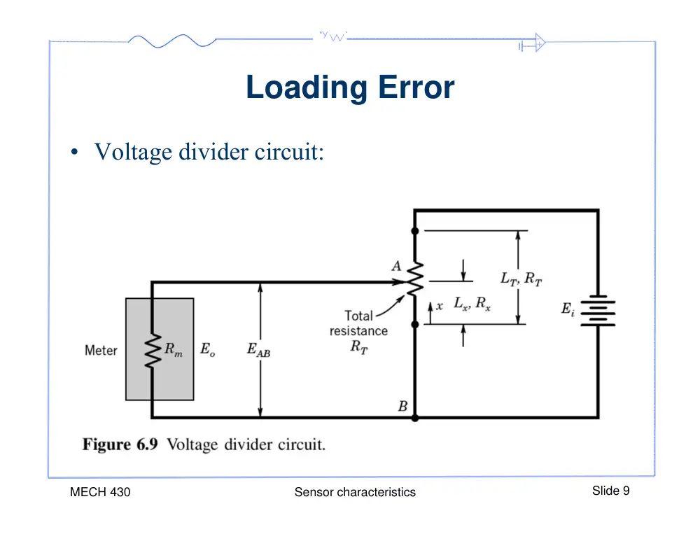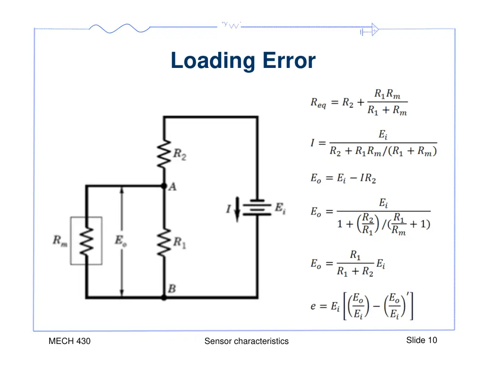MECH 430 Sensor characteristics Slide 8 Loading Error • Voltage divider circuit: MECH 430 Sensor characteristics Slide 9 Loading Error MECH 430 Sensor characteristics Slide 10 6.4 Bridge Circuits • Bridge circuits have been devised for measurement of capacitance, inductance and most often for Resistance measurement. • Resistive bridge is called Wheatstone Bridge provides means for accurately measuring resistance, and detecting small resistance changes. MECH 430 Introduction Slide 11 MECH 430 SC_Bridge_circuits Slide 12 Resistive Bridge Circuit • Resistive bridge circuits are used in measurement of temperature, pressure, strain, force, magnetic fields… • One or more legs may be a thermistor, strain gauge, RTD, piezoresistive element, potentiometer, … • The input excitation VR can be ac or dc. MECH 430 SC_Bridge_circuits Slide 13 The balanced condition • If Rm>> all R’s, the bridge acts like an open circuit and im = 0. 3 2 2 4 1 1 R R V i R R V i R R     R CB R AB R V R R i R V R V R R i R V 3 2 2 2 2 4 1 1 1 1       CB AB BC AB AC o V V V V V V      (1) (2) (3) (4) (5) Vo MECH 430 SC_Bridge_circuits Slide 14 The balanced condition • Subbing (3) & (4) into (5) gives:    R o R V R R R R R R R V 3 2 4 1 4 2 1 3     If Vo = 0 then R1R3 = R2R4 k R R R R   3 2 4 1 (6) (7) Condition for a balanced bridge MECH 430 SC_Bridge_circuits Slide 15 Operating modes of bridge circuits • Bridges may be operated in deflection (unbalanced) mode, or null-balanced mode. Vo R2 R3 Rx R4 VR B D A C MECH 430 SC_Bridge_circuits Slide 16 The unbalanced mode • Starting from a balanced state, if the sensor resistance Rx changes by x, a voltage across the bridge diagonal is generated (i.e., V0 ≠ 0). • Vo can be used to compute this change using a calibrated meter. • Vo is a nonlinear function of unbalance x. This method is suitable for small changes in resistors (x < 0.005). The unbalanced mode MECH 430 Introduction Slide 17    R o R V R R R R R R R V 3 2 4 1 4 2 1 3     MECH 430 SC_Bridge_circuits Slide 18 The null-balanced mode • This mode requires that the bridge is always maintained at a balanced state (i.e., Vo = 0). • To satisfy this condition, we have to vary one of resistor (e.g., R2) by a control circuit based on the change in Rx. • Any change in Rx causes a meter deflection and an error signal is generated by a control circuit which modifies R2 until its effect cancels that of Rx and the bridge is balanced again. • The advantages of this method is that the input voltage need not be known, and current detector is needed instead of a current sensor. Example 6.3 • A Temp sensor changes it resistance with temp according to: – R is current sensor resistance – R0 is sensor resistance at T0 – T is current temperature – T0 is temperature reference at 0ºC – Alpha is constant = 0.00395ºC-1 • It is connected to a deflection bridge at the R1 location where initially all arms are equal to 100Ω. The supply voltage is 10V. • If the temperature of R1 is changed so that Vo is equal to 0.569V, What is the temp of the sensor? MECH 430 Introduction Slide 19 MECH 430 SC_amplification Slide 20 6.6 Signal Amplification • The simplest form of signal processing is signal amplification. • The need arises because transducers provide signal that are said `weak’ (i.e, μV or mV), and are too small for reliable processing. • Standard electronics data processors (A/D, frequency modulators) require signals of sizeable amount (Volts and mA). MECH 430 SC_amplification Slide 21 6.6 Signal Amplification • Usually the raw signal is multiplied by a constant: – Voltage gain AV up to 1000, – Current gain AI up to 106. • Amplification maximizes the use of available voltage range to: – Increase accuracy, – Increase Signal to Noise Ratio (SNR). MECH 430 SC_amplification Slide 22 Linearity & Distortion • Linearity in amplifiers is important, such that when we feed a signal to an amplifier, we want the output signal of the amplifier to be an exact replica of the input, except of course for having a larger amplitude. • Any change in waveform is considered to be a distortion, and is undesirable. MECH 430 SC_amplification Slide 23 Linearity & distortion • An amplifier that preserves the relationship between input and output is called a linear amplifier and is characterized by: ( ) ( ) Av t t v i o  • If this relationship contains higher powers of vi then the amplifier is said to exhibit nonlinear distortion. Amplifier gain MECH 430 SC_amplification Slide 24 Signal Amplification • The amplification discussed so far operate on small input signals and are known as voltage amplifiers (will be used here). • Another type of amplifier is the power amplifier that provides a modest amount of voltage gain but substantial current gain. • Power amplifiers absorb little power from the input but deliver large amounts of power to its load. MECH 430 SC_amplification Slide 25 The raw signal generated by most passive sensors may be in the order of mV or nA. A thermocouple with one iron arm (high emf at +3.54mV) and one nickel arm (low emf at – 3.1mV) produces an output of 6.64 mV for ∆T =200oC. A photodiode has a current output of 10μA when illuminated and 10nA in total darkness. Typical signal range of common sensors CF is added to provide noise filtering. CF RF i i F out iR V   Sensing junction Material 2 Material 1 Reference MECH 430 SC_amplification Slide 26 Operational Amplifier (Op-amp) • The first types of op-amps were constructed from vacuum tubes and then transistors and resistors, but built separately. • The first Integrated Circuit (IC) op-amp was manufactured in the 1960. In this chip, all resistors and transistors were integrated onto a single silicon chip. • A nice feature about op-amps is that they operate at levels close to their predicted theoretical performance. • Op-amps will be studied in this course as a black boxes (i.e., we will not study their internals), where we will study how they are used in circuits. OP-AMP Applications MECH 430 Introduction Slide 27 Operational Amplifier MECH 430 Introduction Slide 28 Operational Amplifier MECH 430 Introduction Slide 29 MECH 430 SC_amplification Slide 30 Op-Amp Terminals • An op-amp has 5 terminals: – 3 terminal for signal flow: 2 inputs(1,2) and 1 output (3), – 2 terminals for power (4,5). • In addition to these terminals an op-amp can have other terminals for specific purposes (e.g., offset nulling, not covered here).   MECH 430 SC_amplification Slide 31 Ideal Op-amp • An ideal op-amp senses the difference between the voltage (with respect to ground) of signals applied at its two terminals (v2-v1) multiplies it by a number A and causes a resulting voltage A(v2-v1) at terminal 3. 1 2 3 + - + v1 v2 +- +- +-  1  2 v A v  Power supply 1  0 i i2  0 MECH 430 SC_amplification Slide 32 Ideal Op-amp • At its inputs: – Draws zero current at its inputs, – The input impedance is infinite. • At its output: – Acts as an ideal voltage source. – This means that regardless of how much current the output load is drawing, the op-amp and keep up and the voltage at the output does not drop. – The output impedance is zero. 1 2 3 + - + v1 v2 +- +- +-  1  2 v A v  Power supply 1  0 i i2  0 MECH 430 SC_amplification Slide 33 Ideal Op-amp • The output voltage is in phase (has the same sign) as the v2 but opposite sign than v1. • For this reason v1 is called the inverting terminal and v2 is called the non-inverting terminal. 1 2 3 + - + v1 v2 +- +- +-  1  2 v A v  Power supply 1  0 i i2  0 MECH 430 SC_amplification Slide 34 Common mode rejection • Note that the op-amp amplifies the difference between the two terminals. Therefore if both terminals are corrupted by similar noise, this noise will not be amplified (beauty of an op-amp). • This property is called common mode rejection. • Note that the gain A is called differential gain (usually of the order of 105 to 106). 1 2 3 + - + v1 v2 +- +- +-  1  2 v A v  Power supply 2  0 i i1  0 MECH 430 SC_amplification Slide 35 Ideal Op-amp 1 2 3 + - + v1 v2 +- +- +-  1  2 v A v  Power supply 1  0 i 2  0 i                      CC n p CC CC n p CC n p CC n p CC o V v ) A(v V V v ) A( v V v ) A(v V v ) A( v V v MECH 430 SC_amplification Slide 36 Ideal Op-amp • Given that the feedforward open loop gain (i.e., from input to output without any looping back) is very large, they are rarely used in open loop. • Rather, op-amps are usually used in feedback, closing the loop around the op-amp. 1 2 3 + - + v1 v2 +- +- +-  1  2 v A v  Power supply 1  0 i i2  0 Ideal Op-Amp • In the linear region of operation of the op-amp: • This golden rule is not valid if the op-amp is operating in the saturated region. • To operate in the linear region, a negative feedback from the output to the inverting input of the op-amp must be present. • If a circuit containing an op amp does not provide a negative feedback path from the op-amp output to the inverting input, then the op-amp will normally saturate • Finally, note that, even with negative feedback, operation in the linear region is not guaranteed! MECH 430 Introduction Slide 37 n p v  v MECH 430 SC_amplification Slide 38 Inverting op-amps • We get an inverting amplifier by: 1) Connecting a resistor in the negative feedback, 2) Connecting a resistor between the voltage source and the op amp negative terminal, 3) Connecting the non-inverted terminal to ground. MECH 430 SC_amplification Slide 39 Closed-loop gain • In this case: v2 ≈ v1. • In such systems we say the two terminals are ``tracking each other in potential’’. • We also speak of a virtual short circuit between the two terminals. • We speak of terminal 1 as being a virtual ground. 0 ) ( 1 2 1 2       A v v v v A v v o o 1i MECH 430 SC_amplification Slide 40 Closed-loop gain • The current through R1 is: 1 1 1 1 R v R v v i i i    • The voltage across R2 is: 2 1 0 R R v v i o   1 2 R R v v i o   • The closed loop gain is: MECH 430 SC_amplification Slide 41 Closed-loop gain • This is a very interesting results and states that we can make the gain of the op-amp as accurate as we want by selecting passive components (i.e., resistors) of appropriate accuracy. • It also means that the closed loop gain of the op- amp is independent of the op amp internal gain. 1 2 R R v v i o   1i MECH 430 SC_amplification Slide 42 Equivalent circuit • The input resistance of the equivalent circuit is found as: + - iv R R 1 2  iv o  0 R + - R1 Ri  1 1 1 R R v v i v R i i i in    • The inverting configuration suffers from a low input resistance.  MECH 430 SC_amplification Slide 43 Other applications of inverting op- amps • If we replace the resistances by impedances: 1 2 Z Z V V i o   MECH 430 SC_amplification Slide 44 Miller Integrator • For instance if we use a resistor and capacitor, the resulting circuit acts as an integrator: jwCR sCR V V i o 1 1     R v t i i ) ( 1  vo(t)  VC  i1(t) 0 t C  vo(t)  VC  1 CR vi(t) 0 t In Laplace: MECH 430 SC_amplification Slide 45 Miller Integrator • This circuit is known as the Miller integrator. • At zero frequency (dc) the gain is infinite and the circuit operates as open loop. vo(t)  VC  1 CR vi(t) 0 t Initial voltage across capacitor Integration time constant MECH 430 SC_amplification Slide 46 Differentiator • If we use the capacitor for Z1 and the resistor for Z2 the circuit acts as a differentiator: jwCR sCR V V i o     dt CR dv t t v i o ( ) ( )   MECH 430 SC_amplification Slide 47 Differentiator • The differentiator circuit is a noise amplifier. • A spike is introduced every time there is a sharp change in vi(t). Such a spike could be picked-up interference. • For this reason differentiator circuits are usually avoided in practice. MECH 430 SC_amplification Slide 48 Weighted Summer • Another application of an inverting op-amp: 3 3 3 2 2 2 1 1 1 , , R v i R v i R v i    f o iR v             3 3 2 2 1 1 v R R v R R v R R v f f f o MECH 430 SC_amplification Slide 49 Weighted summer, opposite signs • To include opposite signs use 2 op-amps: vo  v1 Ra R1     Rc Rb      v2 Ra R2     Rc Rb      v2 Rc R3      v4 Rc R4     MECH 430 SC_amplification Slide 50 Non-inverting op-amp • In a non-inverting op-amp the input signal is applied to the positive terminal, while the negative terminal is connected to ground. 1 1 R v i i  0 1 2    A v v v o 1 2 2 1 1 R R v v R R v v v i o i i o            MECH 430 SC_amplification Slide 51 Non-inverting amplifier • The property of infinite input impedance enables using the circuit as a buffer amplifier, where a source with high impedance connects to a load with low impedance. • The buffer amplifier is used as an impedance transformer. + - iv R R        1 2 1 iv o  0 R + -   iR  MECH 430 SC_amplification Slide 52 Buffer op-amp • The buffer amplifier can also be constructed by making R2 = 0 and R1 = ∞. • This circuit is referred to as a voltage follower, since the output follows the input. MECH 430 SC_amplification Slide 53 Difference Amplifier • We need to find the expression of the output voltage vo in terms of the input voltages v1 and v2. Difference Amplifier MECH 430 Introduction Slide 54 Difference Amplifier MECH 430 Introduction Slide 55 MECH 430 SC_amplification Slide 56 Problem with a difference amplifier • Looking at the difference voltage supply • The resistance seen by vId is called the differential input resistance RId • A drawback of a difference amplifier is that RId is finite RId  vId i1 vId  R1i1  0  R1ii RId  2R1 Loop equation: MECH 430 SC_amplification Slide 57 Instrumentation amplifier • A much better type of instrumentation amplifier is shown below. • The circuit consists of two stages: – Stage 1: Two op-amps with three resistors, – Stage 2: One difference amplifier. Instrumentation amplifier MECH 430 Introduction Slide 58 MECH 430 SC_amplification Slide 59 Instrumentation amplifier • The virtual short circuits at the inputs of op-amps A1 and A2 cause the voltages v1 and v2 to appear at the two terminals of the resistor R1. • A current i = (v1-v2)/2R1 flows through 2R1 and the two resistors R2. MECH 430 SC_amplification Slide 60 Instrumentation amplifier • Any common-mode signal vCM results in NO current flowing through R1 and therefore vo1= vo2= 0. • The second stage amplifier senses No voltage gradient and produces zero output voltage. Amplification Difference