MECH 430 Notes 5, Spring 2014

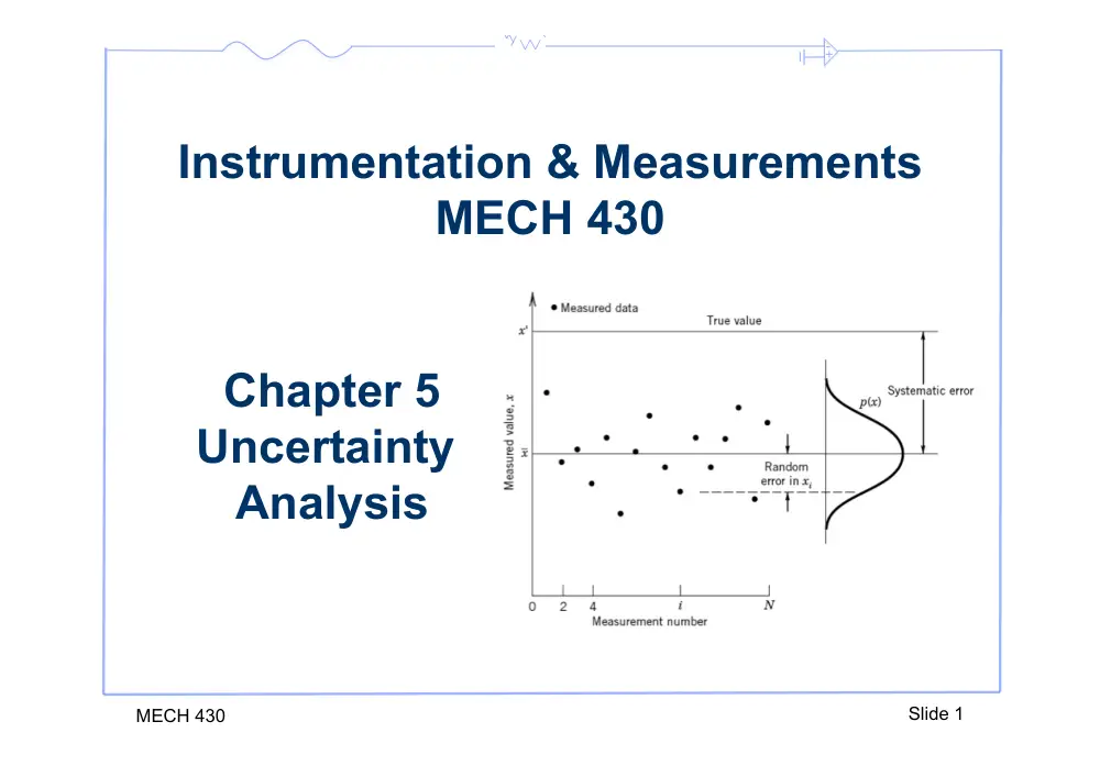
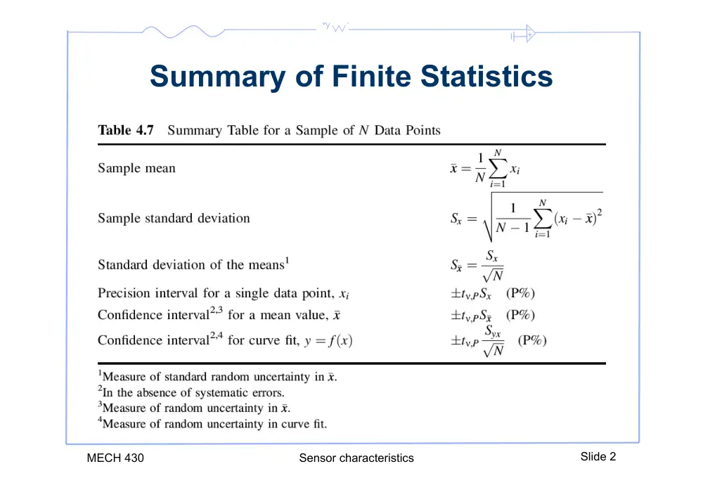
- + Instrumentation & Measurements MECH 430 MECH 430 Slide 1 Chapter 5 Uncertainty Analysis - + Summary of Finite Statistics MECH 430 Sensor characteristics Slide 2 - + MECH 430 Slide 3 5.1 Introduction • Uncertainty analysis provides a methodical approach to estimating the accuracy of results. • In other words we can estimate the “±what” in a planned test. • Errors causes a difference from the true value, but since we don’t know the true value and hence we estimate a range of probable error. This estimate is called uncertainty. • Uncertainty is a property of the result. - + 5.1 Introduction •  The uncertainty describes an interval about the measured value within which we suspect that the true value must fall with a stated probability. •  What we want to do is quantify, on average, how closely the measured value agrees with some known true value and base our interpretation of subsequent measured results on that information. •  Uncertainty quantifies the quality of the result. MECH 430 Sensor characteristics Slide 4 - + 5.2 Measurement Errors •  An error is the difference between a measured value and the true value. An error is a property of a measurement. •  Errors are introduced from various elements: –  The instrument, –  The data set finite statistics, –  The approach used. •  Given that we can not know the true value, we can estimate a range of probable error. •  We call this estimate the uncertainty. •  Uncertainty analysis is the process of identifying, quantifying, and combining these errors. 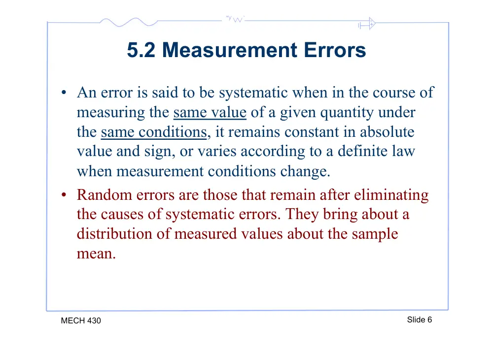MECH 430 Slide 5 - + MECH 430 Slide 6 5.2 Measurement Errors •  An error is said to be systematic when in the course of measuring the same value of a given quantity under the same conditions, it remains constant in absolute value and sign, or varies according to a definite law when measurement conditions change. •  Random errors are those that remain after eliminating the causes of systematic errors. They bring about a distribution of measured values about the sample mean. - + Systematic & Random Errors MECH 430 Slide 7 •  The systematic errors will shift the sample mean from the true mean of the measured variable by a fixed amount. •  The random errors bring about a distribution of measured values about the sample mean. 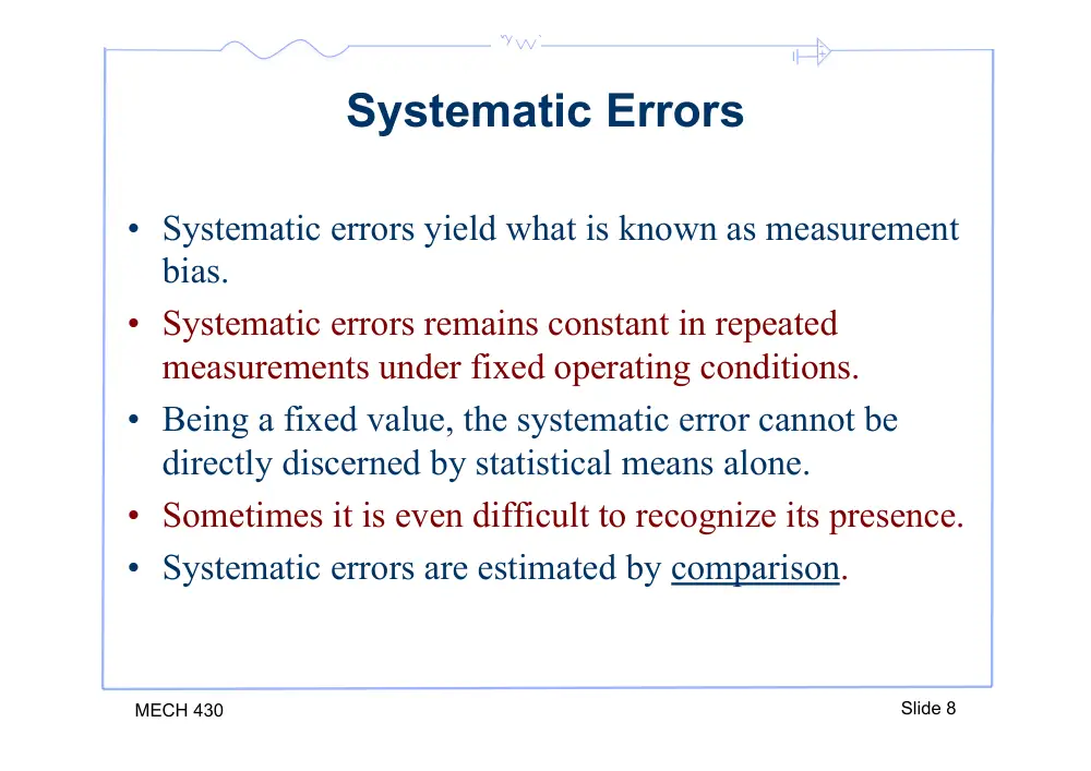- + MECH 430 Slide 8 Systematic Errors •  Systematic errors yield what is known as measurement bias. •  Systematic errors remains constant in repeated measurements under fixed operating conditions. •  Being a fixed value, the systematic error cannot be directly discerned by statistical means alone. •  Sometimes it is even difficult to recognize its presence. •  Systematic errors are estimated by comparison. 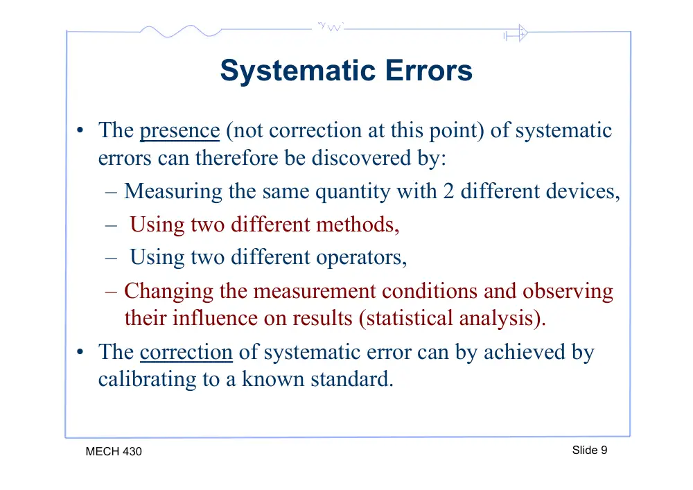- + MECH 430 Slide 9 Systematic Errors •  The presence (not correction at this point) of systematic errors can therefore be discovered by: –  Measuring the same quantity with 2 different devices, –  Using two different methods, –  Using two different operators, –  Changing the measurement conditions and observing their influence on results (statistical analysis). •  The correction of systematic error can by achieved by calibrating to a known standard. - + Random Errors •  Random error, also called precision error, is affected by the repeatability and resolution of the measurement system components. •  Because of the varying nature of the random errors, exact values cannot be given, but probable estimates of the error can be made through statistical analyses. MECH 430 Slide 10 - + MECH 430 Slide 11 Random Errors •  Random errors are characterized by the following: –  Positive and negative random errors with the same absolute values have the same occurrence probability. –  The probability of occurrence of a random error decreases as its absolute value increases. - + MECH 430 Slide 12 Random Errors •  In the absence of systematic errors, the best estimate of the actual value of a measurand is obtained by taking n measurements and averaging the results: n x x x x n n + + + =  2 1 ˆ •  When n is infinite, (1.3) yields the true value for x. •  However, when n is finite, each experiment that yields a group of x’s gives a different average. •  The random uncertainty at a defined confidence level is defined by the interval - + 5.3 Design Stage Uncertainty •  Analysis done prior to measurement. •  It is useful for selecting instruments, measurement techniques, and estimating the likely uncertainty to exist in the measured data. •  Data at this level is obtained from catalogues. •  It is probably difficult in this stage to distinguish between systematic and random errors. •  The goal of the design stage is to estimate the magnitude of uncertainty in the measured value that would result from a measurement. MECH 430 Slide 13 - + 5.3 Design Stage Uncertainty •  The zero-order uncertainty (u0) of an instrument reflects our ability to resolve the information provided by the instrument. •  At zero-order uncertainty we assume the variation expected in the measured values will be that of the instrument resolution alone and all other aspects of the measurement are perfectly controlled. •  u0 is an estimate of the expected random uncertainty caused by the data scatter due to reading the instrument. MECH 430 Slide 14 - + Zero-order Uncertainty •  As a rule of thumb, assign a numerical value to u0 of one half of the instrument resolution with a probability of 95%. MECH 430 Slide 15 u0 = ± 1 2 resolution (95%) •  At 95%, we assume that only one measured value in 20 will have a value outside of u0. - + Instrument Uncertainty •  The second piece of information from a manufacturer is the instrument uncertainty uc •  Essentially, uc is an estimate of the systematic error for the instrument. •  Sometimes the instrument error will be stated in parts, each part due to some contributing factor. •  We combine these errors via the root-sum-squares (RSS) method. MECH 430 Slide 16 - + MECH 430 Slide 17 Root Sum Square (RSS) method •  We will refer to each individual error as an elemental error. •  For example the sensitivity error and the linearity error of a transducer are two elemental errors. •  Consider a measurement of x subject to k elemental errors e1,e2,…en: ux = ± e1 2,e2 2,,eK 2 = ± ek 2 k=1 K ∑ - + Different type of instrument errors: - Hysteresis - Linearity - Sensitivity - Zero Shift - Repeatability MECH 430 Slide 18 - + RSS method •  In calculating RSS be careful to be consistent with the units. •  Furthermore, each error should be estimated at the same probability level. A general rule is to use 95%. •  If no probability level is provided on the datasheet, a 95% level can be assumed. MECH 430 Slide 19 - + 5.3 Design Stage Uncertainty •  The design stage uncertainty is then obtained by combining the instrument uncertainty with the zero- order uncertainty: MECH 430 Slide 20 ud = u0 2 + uc 2 •  The design stage uncertainty is used as a guide for selecting equipment and is NOT the final estimate of the total uncertainty in a measurement system. •  If additional information is known at this stage then should be included in the above equation. - + 5.3 Design Stage Uncertainty MECH 430 Sensor characteristics Slide 21 - + Example 5.1 •  Given: a force measuring instrument is described by the catalogue data below. •  Estimate: the uncertainties attributable to this instrument and the instrument design stage uncertainty. MECH 430 Slide 22 Resolution 0.25N Range 0 to 100N Linearity within 0.2 N over range Hysteresis within 0.3N over range - + Example 5.1 •  Solution: first find elemental errors of linearity and hysteresis MECH 430 Slide 23 ulinearity = 0.2N uhysteresis = 0.3N •  Next combine using RSS to find uc: uc = ± 0.22 + 0.32 = ±0.36N (95%) •  The instrument resolution is 0.25N so u0 = ±0.125N •  Finally the design-stage uncertainty is: ud = ± u0 2 + uc 2 = ± 0.362 + 0.1252 = ±0.38N (95%) - + Example 5.2 •  Given: a voltmeter is to be used to measure the output of a pressure transducer. •  Pressure transducer (3psi expected nominal pressure) –  Range: ±5psi –  Sensitivity: 1V/psi –  Input power: 10VDC ±1% –  Output: ±5V –  Linearity: within 2.5mV/psi over range –  Sensitivity: within 2mV/psi over range –  Resolution: negligible MECH 430 Slide 24 - + Example 5.2 •  Voltmeter –  Resolution: 10µV –  Accuracy: within 0.001% reading •  Find: –  uc for each device –  ud for the measurement MECH 430 Slide 25 - + Example 5.2 •  Solution: MECH 430 Slide 26 The design stage uncertainty for the voltmeter is: (ud )E = ± (u0 )E 2 + uc ( )E 2 = ±30.4µV (95%) (u0 )E = ±5µV (95%) (uc )E = ± 3V × 0.00001 ( ) = ±30µV (95%) - + Example 5.2 •  Solution: MECH 430 Slide 27 The design stage uncertainty for the pressure transducer is: (ud )E = ± (u0 )E 2 + uc ( )E 2 = ±9.61mV (95%) (u0 )P = 0 (uc )P = ± (2.5mV / psi × 3psi ) 2 + 2mV / psi × 3psi ( ) 2 = ±9.61mV (95%) - + Example 5.2 •  Solution: MECH 430 Slide 28 Finally, the design stage uncertainty for the entire system is: ud = ± (ud )E 2 + ud ( )P 2 = ± (0.030mV ) 2 + 9.61mV ( ) 2 = ±9.61mV (95%) Using the sensitivity of 1V/psi, the uncertainty in psi is: ud = ±0.0096psi (95%) - + 5.4 Error Sources •  Design-stage uncertainty does not address all possible errors. •  If we consider the measurement process to consist of 3 steps, and each has an uncertainty associated with it: –  calibration error, –  data-acquisition error, –  data reduction error. MECH 430 Slide 29 - + 5.4 Error Sources MECH 430 Slide 30 Calibration errors DAQ errors Data reduction errors - + 5.6 Error Propagation •  Very often results are obtained through a functional relationship with measured values. •  For example the measurement of flow rate using time and volume. Q = f( t, V) •  How do uncertainties in either quantity contribute to uncertainty in flow rate? •  Is the uncertainty in Q more sensitive to uncertainty in t or v? •  How are errors propagated to a calculated result? MECH 430 Slide 31 - + 5.6 Error Propagation •  The true value of y falls within the interval MECH 430 Slide 32 y ± δy = f (x ± tSx ) - + 5.6 Error Propagation •  Expanding using a Taylor series: MECH 430 Slide 33 y ± δy = f (x ± tSx ) y ± δy = f (x) ± dy dx " #$ % &' x= x tSx + 1 2 d 2y dx2 " #$ % &' x= x (tSx ) 2 + ( ) * * + , - - •  If is small and if we neglect higher order terms: tSx δy ≈ dy dx # $% & '( x= x tSx - + 5.6 Error Propagation •  From above the uncertainty for the dependent variable is related to the uncertainty in the independent variable by: MECH 430 Slide 34 uy = dy dx ! "# $ %& x= x ux - + Multiple Variables •  For multiple variables with R = f1(x1, x2, …, xL) the best estimate for the true mean R’ is: MECH 430 Slide 35 R' = R ± uR (P%) R = f1(x1,x2,,xL) uR = ± (θiuxi ) 2 i=1 L ∑ # $% & '( 1/2 (P%) θi = ∂R ∂xix=x i = 1,2,...,L - + Example 5.3 •  Given: –  A displacement sensor has a calibration curve y = KE, –  E = 5V, –  K = 10.10 mm/V –  uK = ±0.10 mm/V (95% confidence) –  uE = ±0.01 V (95% confidence) •  Find: –  The uncertainty in displacement MECH 430 Slide 36 - + Example 5.3 •  Solution MECH 430 Slide 37 y = f (E,K) uy = f (uE,uK ) •  The uncertainty is found as: uy = ± (θEuE ) 2 + θKuK ( ) 2 "# $% 1/2 θE = ∂y ∂E = K θK = ∂y ∂K = E •  Therefore: uy = ± (K(0.01) ) 2 + E(0.1) ( ) 2 !" #$ 1/2 = ±0.51mm (95%) - + Sequential Perturbation •  It might be difficult to find the partial derivatives in the previous method. •  We then resort to something known as sequential perturbation. •  This method is based on using a finite difference method to approximate the derivatives. MECH 430 Slide 38 - + Sequential Perturbation •  Start by finding an operating point Ro= f(x1, x2,…, xL) •  Next, increase the independent variables by their uncertainties to find MECH 430 Slide 39 Ri + R1 + = f (x1 + ux1,x2,...,xL), R2 + = f (x1,x2 + ux2 ,...,xL),... RL + = f (x1,x2,...,xL + uxL ) •  Do the same to find •  Calculate the differences: Ri − δRi + = Ri + − Ro δRi − = Ri − − Ro - + Sequential Perturbation •  Finally find the approximate uncertainty contribution of each variable. MECH 430 Slide 40 •  The uncertainty is then calculated as: uR = ± (δRi ) 2 i=1 L ∑ # $% & '( 1/2 (P%) δRi = δRi + − δRi − 2 ≈ θiui - + Example 5.3 (continued) •  Alternatively we can use sequential perturbation with Ro = 50.5 mm MECH 430 Slide 41 •  The uncertainty is found as: uy = ± (0.10 ) 2 + 0.5 ( ) 2 !" #$ 1/2 = ±0.51mm •  Therefore the displacement is: y' = 50.50 ± 0.51mm (95%) i xi 1 E 50.60 50.40 0.1 -0.1 0.1 2 K 51.00 50.00 0.5 -0.5 0.5 Ri + Ri − δRi + δRi − δRi - + MECH 430 Slide 42 Principle of equal effects • If you have the total uncertainty and want to find each individual uncertainty, we can use the principal of equal effects. • This principal states that each source of uncertainty ∆ui contributes an equal amount to the total uncertainty ∆R. ( ) i i u R n R u ∂ ∂ Δ = Δ / (1) - + MECH 430 Slide 43 Example •  A dynamometer is used to measure the average power output on a shaft. t RFL P 12 550 2 × = π Time of run (s) Number of revolutions of the shaft during t seconds Force at the end of the torque arm (lbf) Length of torque arm (ft) Average power (hp) K - + MECH 430 Slide 44 Example •  Given: –  For a given run we have the following measurements with their associated errors –  Find the overall uncertainty: .0 55 s .00 60 .0 05 in .63 15 .0 04 lbf .12 10 1rev 1202 ± = ± = ± = ± = t L F R - + MECH 430 Slide 45 Example • Solution: – Find the partial differentials: 051 hp/s .0 193 hp/in .0 0251 hp/rev .0 298 hp/lbf .0 2 = − ∂ = ∂ = = ∂ ∂ = = ∂ ∂ = = ∂ ∂ t KFLR t P t KFR L P t KFL R P t KLR F P F = 10.12 ± 0.04 lbf R = 1202 ±1 rev L = 15.63 ± 0.05 in t = 60.00 ± 0.55 s - + MECH 430 Slide 46 Example • The overall uncertainty is found as: ΔRRSS = (0.04 × 0.298 ) 2 + 1× 0.00251 ( ) 2 + 0.05 × 0.193 ( ) 2 + 0.55 × 0.05 ( ) 2 = .0 029 hp Δ RSS R • The power is calculated as: = .3 016 hp = t KFLR P •  If we wish to measure P to within 0.5% uncertainty, what are the errors associated with each individual measurement? - + MECH 430 Slide 47 Example ΔF = ΔP n ∂P / ∂F ( ) = 0.005 × 3.016 4 0.298 ( ) = 0.013 lbf ΔR = ΔP n ∂P / ∂R ( ) = 0.005 × 3.016 4 0.00251 ( ) = 1.5 rev ΔL = ΔP n ∂P / ∂F ( ) = 0.005 × 3.016 4 0.193 ( ) = 0.019 in Δt = ΔP n ∂P / ∂F ( ) = 0.005 × 3.016 4 0.05 ( ) = 0.075 s •  Using the principle of equal effects: - + 5.7 Advanced Stage Uncertainty •  Higher order uncertainty considers the controllability of test operating conditions and the variability of all measured variables. •  For example, at a first order level, the effect of time as an extraneous variable could be considered. MECH 430 Slide 48 uN = uc 2 + ( ui 2 i=1 N −1 ∑ ) # $ % % & ' ( ( 1/2 (P%) u0 = ± 1 2 resolution u1 = ±t J −1 ( ),95ST - + Example 5-4 •  Examine a dial oven thermometer and assess the zero and first order uncertainties if we have J measurements MECH 430 Slide 49 u0 = ± 1 2 resolution u1 = ±t J −1 ( ),95ST - + Example •  A stopwatch is to be used to estimate the time between the start and end of an event. Event duration might range from several seconds to 10 minutes. Estimate the probable uncertainty in a time estimate using a stopwatch that claims an accuracy of 1 minute per month and a resolution of 0.01 seconds. MECH 430 Sensor characteristics Slide 50 - + Example •  Zero stage uncertainty MECH 430 Sensor characteristics Slide 51 u0 = ±0.01/ 2s uc = ± 60s 1(30)(24)(60)(60)s T T =10s ⇒ ud = ± u0 2 +uc 2 = ± 0.0052 + 10 60 1(30)(24)(60)(60) " #$ % &' 2 = ±0.005s T =10min = 600s ⇒ ud = ± u0 2 +uc 2 = ± 0.0052 + 10(600) 60 1(30)(24)(60)(60) " #$ % &' 2 = ±0.015s - + Example •  Now assume that the operator takes some time to detect the start and end of the event. Assume this uncertainty is quantified as 150ms with 95% probability. MECH 430 Sensor characteristics Slide 52 u0 = ±0.01/ 2s uc = ± 60s 1(30)(24)(60)(60)s T u1 = ±0.150s t =10s ⇒ uN = ± u1 2 +uc 2 = ± 0.152 + 10 60 1(30)(24)(60)(60) " #$ % &' 2 = ±0.15s t =10min = 600s ⇒ uN = ± u1 2 +uc 2 = ± 0.152 + 10(600) 60 1(30)(24)(60)(60) " #$ % &' 2 = ±0.151s - + Example •  First stage uncertainty is more important (bigger) than the instrument uncertainty. For what duration is this true? MECH 430 Sensor characteristics Slide 53 uc = ± 60s 1(30)(24)(60)(60)s T u1 = ±0.150s T = ??? ⇒ uN = ± u1 2 +uc 2 = ± 0.152 + T 60 1(30)(24)(60)(60) " #$ % &' 2 T 60 1(30)(24)(60)(60) > 0.15 ⇒ t >1.8hrs - + 5.8 Multiple Measurement Uncertainty •  This is applicable if we are able to obtain multiple measurement for each variable of our experiment. •  The propagation of random uncertainty: MECH 430 Slide 54 P = (P1 2 + P2 2 +PK 2)1/2 •  The propagation of elemental systematic error is: standard random uncertainty of each measurement B = (B1 2 + B2 2 +BK 2 )1/2 systematic uncertainty of each measurement - + 5.8 Multiple Measurement Uncertainty •  The total uncertainty is then: MECH 430 Slide 55 ux = ± B2 + tv,95P ( ) 2 ( ) 1/2 (95%) v = Pk 2 k=1 K ∑ " #$ % &' 2 Pk ( 4 / vk ) k=1 K ∑ •  v is found via the Welch-Satterthwaite formula: - + 5.8 Multiple Measurement Uncertainty MECH 430 Sensor characteristics Slide 56 - + Example 5.12 •  Measuring stress in a loaded beam we observe three sources of uncertainty as follows: MECH 430 Slide 57 •  If the mean value of stress is 223.4N/cm2 •  Determine the best estimate of stress at 95% confidence B1 = 1.0N/cm2 B2 = 2.1N/cm2 B3 = 0 N/cm2 P1 = 4.6N/cm2 P2 = 10.3N/cm2 P3 = 1.2N/cm2 v1 = 14 v2 = 37 v3 = 8 - + Example 5.12 •  The random uncertainty is: MECH 430 Slide 58 P = (P1 2 + P2 2 +PK 2)1/2 = 11.3N / cm2 •  The systematic uncertainty is: B = (B1 2 + B2 2 +BK 2 )1/2 = 2.3N / cm2 •  The degree of freedom is: v = Pk 2 k=1 3 ∑ " #$ % &' 2 Pk ( 4 / vk ) k=1 3 ∑ ≈ 49 - + Example 5.12 •  t49,95 = 2 and the uncertainty estimate is: MECH 430 Slide 59 •  The best estimate of a result is: uσ = ±[B2 + tv,95P ( ) 2]1/2 = ±[2.32 + 2 ×11.3 ( ) 2]1/2 = ±22.7N / cm2 σ ' = 223.4 ± 22.7N / cm2 (95%) - + Propagation of Uncertainty •  If we have a function f(x1, x2,…,xn), the true value can be expressed as: MECH 430 Slide 60 R' = R ± uR (P%) R = f1 x1,x2,xL ( ) uR = ± BR 2 + tv,95PR ( ) 2 ( ) 1/2 (95%) BR = "#θiBxi $% 2 i=1 L ∑ ' () * +, 1/2 PR = "#θiPxi $% 2 i=1 L ∑ ' () * +, 1/2 v = θiPxi 2 k=1 K ∑ # $% & '( 2 (θiPxi ) 4 / vxi ( ) k=1 K ∑