CMPS 251 Final, Fall 2005

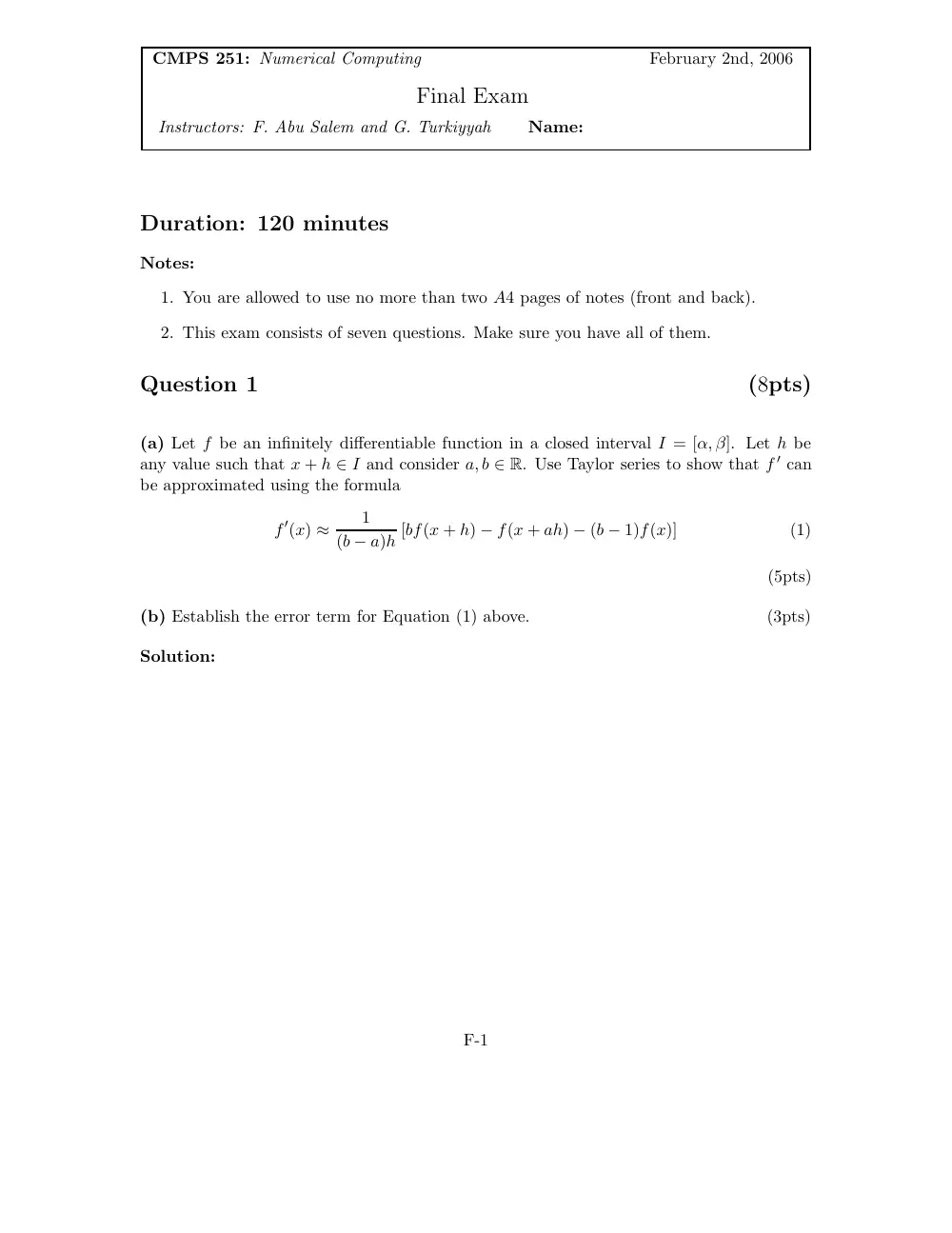
CMPS 251: Numerical Computing February 2nd, 2006 Final Exam Instructors: F. Abu Salem and G. Turkiyyah Name: Duration: 120 minutes Notes: 1. You are allowed to use no more than two A4 pages of notes (front and back). 2. This exam consists of seven questions. Make sure you have all of them. Question 1 (8pts) (a) Let f be an infinitely differentiable function in a closed interval I = [α, β]. Let h be any value such that x + h ∈ I and consider a, b ∈ R. Use Taylor series to show that f ′ can be approximated using the formula f ′(x) ≈ 1 (b − a)h [bf(x + h) − f(x + ah) − (b − 1)f(x)] (1) (5pts) (b) Establish the error term for Equation (1) above. (3pts) Solution: F-1 Solution cont’d: F-2 Question 2 (9pts) Consider the following system of equations:    x1 + αx2 − 3x3 = 7 12x1 + 12αx2 + x3 = 121 αx1 + 4x2 + 2x3 = 6 where α ∈ R. For which values of α does the above system possess 1. no solution? (3pts) 2. infinitely many solutions? (3pts) 3. a unique solution (to be determined if it exists)? (3pts) Solution: F-3 Solution cont’d: F-4 Question 3 (21pts) A symmetric pentadiagonal system is a pentadiagonal system in which the subdiagonals are the same as the superdiagonals. (a) Develop a pseudo-code to solve a symmetric pentadiagonal system using scaled partial pivoting. (7pts) (b) Determine the operational count (run-time in terms of the input size) of your pseudo- code. (7pts) (c) Is this more efficient than the pseudo-code for solving general pentadiagonal systems? Justify your answer in terms of operational and/or spatial costs, whenever applicable. (7pts) Solution: F-5 Solution cont’d: F-6 Question 4 (18pts) (a) What is the minimum number of sub-intervals required to insure that the error in approximating � 2 1 ln x3dx using the trapezoid rule is less than 5 × 10−5? (5pts) (b) Consider the integral � 1 0 exdx. • Use the trapezoid rule to find the value of the integral with 2, 4, and 8 sub-intervals. (5pts) • Use Romberg integration to obtain the best approximation of the integral from the results above. (5pts) • What is the order of the approximation of the Romberg rule above? (i.e., what is the value of k if the error is written as O(hk) where h is the interval size). 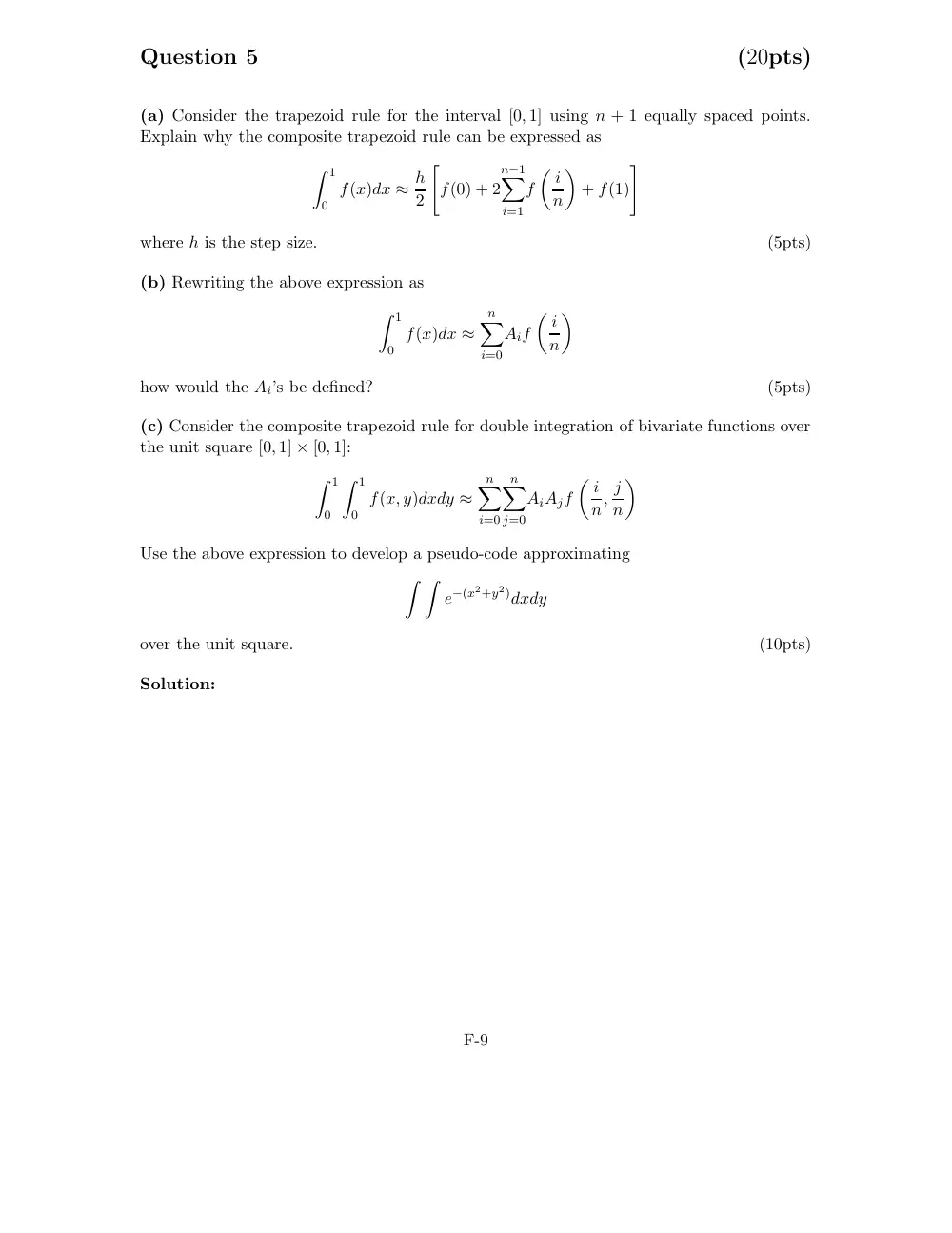(3pts) Solution: F-7 Solution cont’d: F-8 Question 5 (20pts) (a) Consider the trapezoid rule for the interval [0, 1] using n + 1 equally spaced points. Explain why the composite trapezoid rule can be expressed as � 1 0 f(x)dx ≈ h 2 � f(0) + 2 n−1 � i=1 f � i n � + f(1) � where h is the step size. (5pts) (b) Rewriting the above expression as � 1 0 f(x)dx ≈ n � i=0 Aif � i n � how would the Ai’s be defined? (5pts) (c) Consider the composite trapezoid rule for double integration of bivariate functions over the unit square [0, 1] × [0, 1]: � 1 0 � 1 0 f(x, y)dxdy ≈ n � i=0 n � j=0 AiAjf � i n, j n � Use the above expression to develop a pseudo-code approximating � � e−(x2+y2)dxdy over the unit square. (10pts) Solution: F-9 Solution cont’d: F-10 Question 6 (12pts) Consider an iterative solution of the following 2 × 2 set of linear equations: �3 1 1 3 � �x1 x2 � = �1 1 � (a) Determine the Jacobi iteration matrix. (4pts) (b) Will Jacobi converge? Why or why not? (4pts) (c) Perform one iteration of Jacobi with the starting value x0 = (0, 0). (4pts) Solution: F-11 Solution cont’d: F-12 Question 7 (12pts) (a) Determine the values of a and b that make the function f(x) = � x2 x ∈ [0, 1] 1 2(x − 1)2 + a(x − 1) + b x ∈ [1, 3] a quadratic spline. (4pts) (b) In class, we considered the problem of interpolating n + 1 data points with co- ordinates (xi, yi), i = 1, · · · , n + 1, using a quadratic spline Q(x). The continuity and smoothness conditions at x allowed us to express the n spline segements as: qi(x) = zi+1 − zi 2(xi+1 − xi)(x − xi)2 + zi(x − xi) + yi, x ∈ [xi, xi+1] where zi+1 = 2 yi+1−yi xi+1−xi − zi, zi = Q′(xi). In order to determine the parameters zi uniquely we needed one additional condition. In class, we imposed z1 = 0 and used it to compute the remaining zi’s. • Explain how you would compute the unknown coefficients zi if the extra condition becomes alternatively z1 = z2. (4pts) • What is the geometric interpretation of this condition? (4pts) Solution: F-13 Solution cont’d: F-14