EECE 210 Chapter 2, Fall 2012

Chapter 2 Basic Circuit Connections and Laws 2.1 Circuit Terminology  Node: junction of two or more circuit elements.  Essential node: junction of three or more circuit elements.  Path: set of one or more adjoining circuit elements that may be traversed in succession without passing through the same node more than once. A path generally has an initial node at its beginning and a final node at its end.  If the initial and final nodes are the same, the path is closed and becomes a loop.  Mesh: a loop that does not enclose any other loop.  Branch: path that connects two nodes.  Essential branch: branch that connects two essential nodes without passing through an essential node. 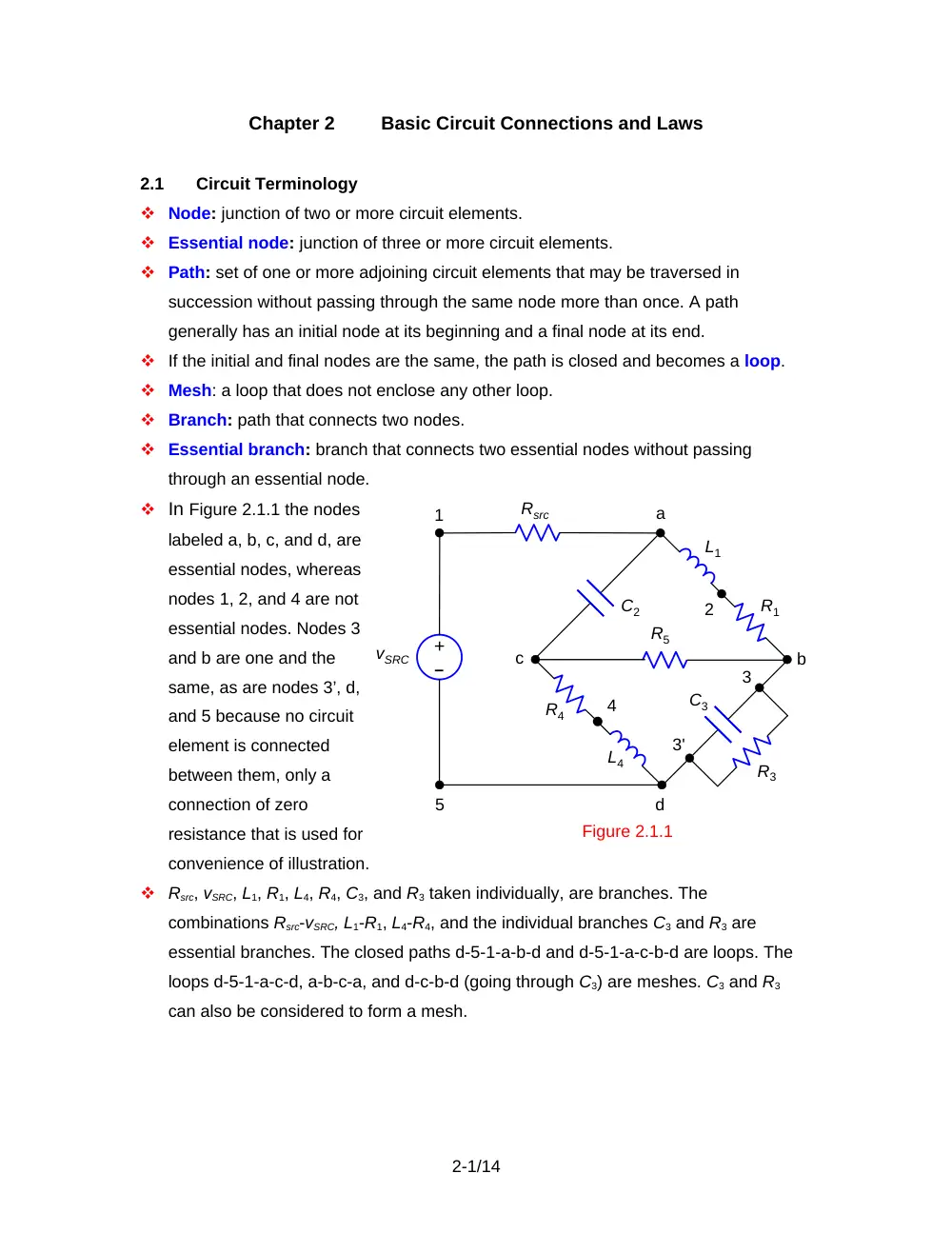 In Figure 2.1.1 the nodes labeled a, b, c, and d, are essential nodes, whereas nodes 1, 2, and 4 are not essential nodes. Nodes 3 and b are one and the same, as are nodes 3’, d, and 5 because no circuit element is connected between them, only a connection of zero resistance that is used for convenience of illustration.  Rsrc, vSRC, L1, R1, L4, R4, C3, and R3 taken individually, are branches. The combinations Rsrc-vSRC, L1-R1, L4-R4, and the individual branches C3 and R3 are essential branches. The closed paths d-5-1-a-b-d and d-5-1-a-c-b-d are loops. The loops d-5-1-a-c-d, a-b-c-a, and d-c-b-d (going through C3) are meshes. C3 and R3 can also be considered to form a mesh. 2-1/14 Figure 2.1.1 L1 vSRC a b c d 1 2 3' 4 R1 R4 L4 R3 C3 R5 C2 – + Rsrc 5 3 2.2 Kirchhoff’s Laws Kirchhoff’s Current Law Statement At any instant of time, the sum of currents entering a node is equal to the sum of currents leaving the node. 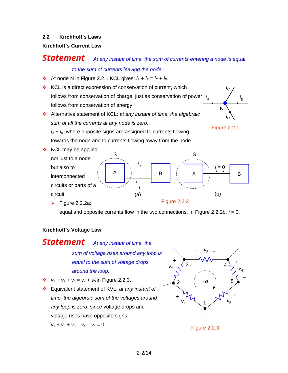 At node N in Figure 2.2.1 KCL gives: iA + iB = iC + iD.  KCL is a direct expression of conservation of current, which follows from conservation of charge, just as conservation of power follows from conservation of energy.  Alternative statement of KCL: at any instant of time, the algebraic sum of all the currents at any node is zero. iA + iB where opposite signs are assigned to currents flowing towards the node and to currents flowing away from the node.  KCL may be applied not just to a node but also to interconnected circuits or parts of a circuit.  Figure 2.2.2a: equal and opposite currents flow in the two connections. In Figure 2.2.2b, i = 0. Kirchhoff’s Voltage Law Statement At any instant of time, the sum of voltage rises around any loop is equal to the sum of voltage drops around the loop.  v1 + v2 + v3 = v4 + v5 in Figure 2.2.3.  Equivalent statement of KVL: at any instant of time, the algebraic sum of the voltages around any loop is zero, since voltage drops and voltage rises have opposite signs: v1 + v2 + v3 – v4 – v5 = 0. 2-2/14 Figure 2.2.1 N iA iC iB iD A B i i (a) A i = 0 B (b) Figure 2.2.2 S S Figure 2.2.3 v1 v5 v2 v4 v3 q + + + + + – – – – – + 1 2 3 4 5 Concept KCL and KVL together are an expression of conservation of energy.  In taking a charge +q clockwise around the loop, the work done on the charge is q(v1 + v2 + v3). But the charge can do more work, q(v4 + v5), if (v1 + v2 + v3) < (v4 + v5), which violates conservation of energy. Taking the charge +q around a loop, which necessarily involves passing through nodes or essentials nodes between the circuit elements, implies that the charge +q is conserved at these nodes, that is, KCL applies. 2.3 Voltage Division and Series Connection of Resistors Definition In a series connection of elements, the same current flows through all the elements. 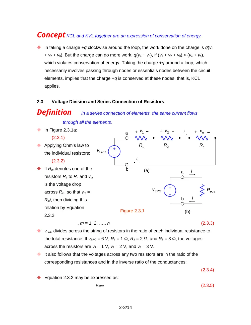 In Figure 2.3.1a: (2.3.1)  Applying Ohm’s law to the individual resistors: (2.3.2)  If Rm denotes one of the resistors R1 to Rn and vm is the voltage drop across Rm, so that vm = Rmi, then dividing this relation by Equation 2.3.2: , m = 1, 2, …., n (2.3.3)  vSRC divides across the string of resistors in the ratio of each individual resistance to the total resistance. If vSRC = 6 V, R1 = 1 , R2 = 2 , and R3 = 3 , the voltages across the resistors are v1 = 1 V, v2 = 2 V, and v3 = 3 V.  It also follows that the voltages across any two resistors are in the ratio of the corresponding resistances and in the inverse ratio of the conductances: (2.3.4)  Equation 2.3.2 may be expressed as: vSRC (2.3.5) 2-3/14 Figure 2.3.1 i Reqs i R1 R2 Rn + v2 – + v1 – + vn – i i a a b b (a) (b) vSRC – + – + vSRC  An equivalent series resistor Reqs is defined such that if vSRC is applied across Reqs, the resulting current is i (Figure 2.3.1b): (2.3.6)  Comparing Equations (2.3.5) and (2.3.6), it follows that: (2.3.7)  In the case of the 1, 2, and 3  resistors connected in series, Reqs = 6 .  Because of the summation of positive quantities in Equation 2.3.7, Reqs is larger than the largest of the individual resistances.  If all the n resistances are equal, Reqs = nR.  If the resistors in Figure 2.3.1a are represented by their conductances, then every resistance in Equation 2.3.7 is replaced by the reciprocal of its reciprocal conductance, which leaves the quantity unchanged. Thus: (2.3.8)  The conductances of the three series-connected 1, 2, and 3  resistors are, respectively, 1, , and S. The sum of their reciprocals is 6 S-1, and S, which is of course the reciprocal of Reqs. Summary In a series connection of resistors, the resistances, or the reciprocals of the conductances, add. 2.4 Current Division and Parallel Connection of Resistors  Definition In a parallel connection of elements, the same voltage is applied across all the elements. 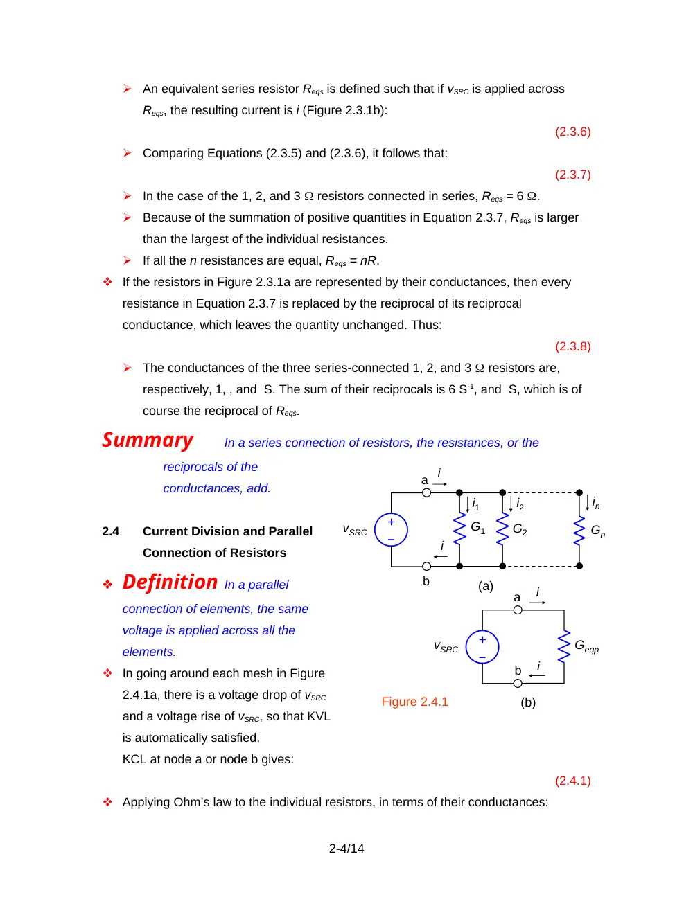 In going around each mesh in Figure 2.4.1a, there is a voltage drop of vSRC and a voltage rise of vSRC, so that KVL is automatically satisfied. KCL at node a or node b gives: (2.4.1)  Applying Ohm’s law to the individual resistors, in terms of their conductances: 2-4/14 Figure 2.4.1 i i i1 i i i2 in Geqp G1 G2 Gn (a) (b) a a b b vSRC – + vSRC – + i1 i i i2 R1 R2 vSRC – + Figure 2.4.2 (2.4.2)  If Gm denotes one of the conductances G1 to Gn, and im is the current through Gm, so that im = GmvSRC, then dividing this relation by Equation 2.4.2: , m = 1, 2, …., n (2.4.3)  i divides between the paralleled resistors in the ratio of each individual conductance to the total conductance. 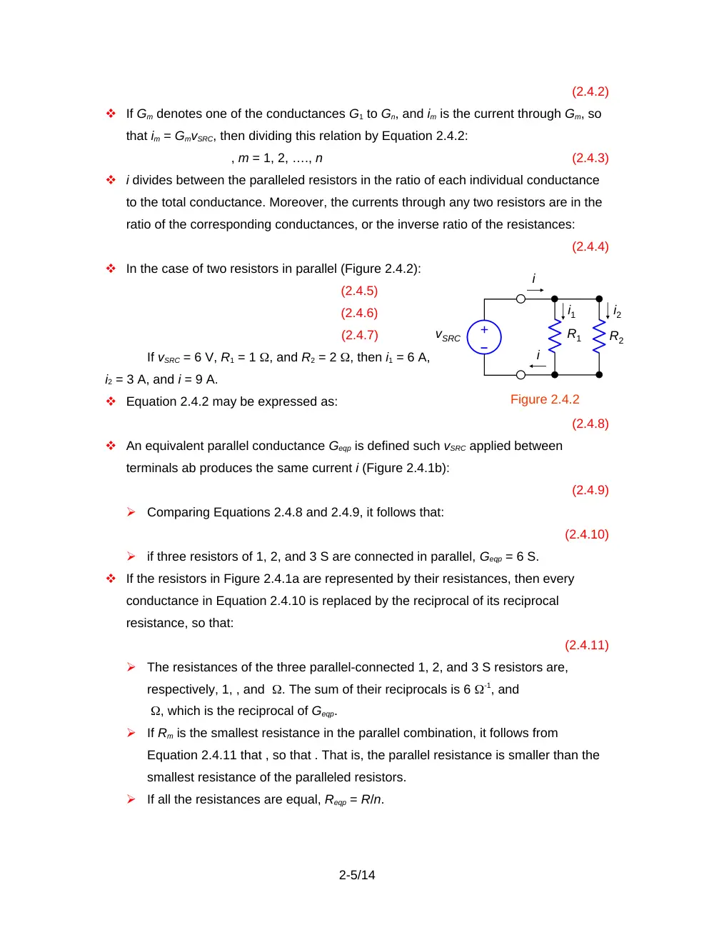Moreover, the currents through any two resistors are in the ratio of the corresponding conductances, or the inverse ratio of the resistances: (2.4.4)  In the case of two resistors in parallel (Figure 2.4.2): (2.4.5) (2.4.6) (2.4.7) If vSRC = 6 V, R1 = 1 , and R2 = 2 , then i1 = 6 A, i2 = 3 A, and i = 9 A.  Equation 2.4.2 may be expressed as: (2.4.8)  An equivalent parallel conductance Geqp is defined such vSRC applied between terminals ab produces the same current i (Figure 2.4.1b): (2.4.9)  Comparing Equations 2.4.8 and 2.4.9, it follows that: (2.4.10)  if three resistors of 1, 2, and 3 S are connected in parallel, Geqp = 6 S.  If the resistors in Figure 2.4.1a are represented by their resistances, then every conductance in Equation 2.4.10 is replaced by the reciprocal of its reciprocal resistance, so that: (2.4.11)  The resistances of the three parallel-connected 1, 2, and 3 S resistors are, respectively, 1, , and . The sum of their reciprocals is 6 -1, and , which is the reciprocal of Geqp.  If Rm is the smallest resistance in the parallel combination, it follows from Equation 2.4.11 that , so that . That is, the parallel resistance is smaller than the smallest resistance of the paralleled resistors.  If all the resistances are equal, Reqp = R/n. 2-5/14 Summary In a parallel connection of resistors, the conductances, or the reciprocals of the resistances, add.  According to Equation 2.4.11, Reqp is the product of the n resistances divided by the sum of their products (n – 1) at a time. 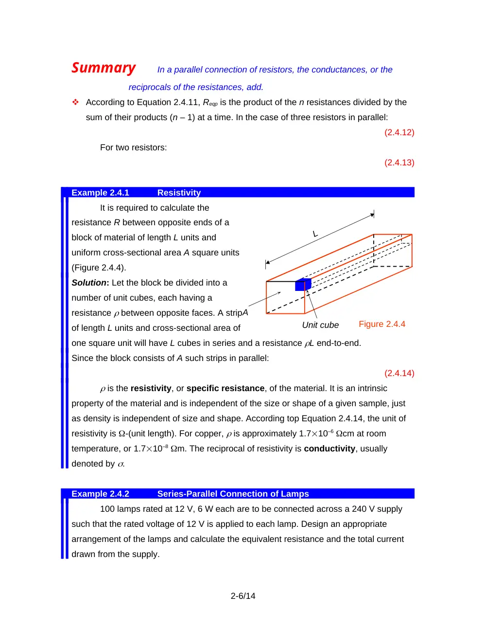In the case of three resistors in parallel: (2.4.12) For two resistors: (2.4.13) Example 2.4.1 Resistivity It is required to calculate the resistance R between opposite ends of a block of material of length L units and uniform cross-sectional area A square units (Figure 2.4.4). Solution: Let the block be divided into a number of unit cubes, each having a resistance  between opposite faces. A strip of length L units and cross-sectional area of one square unit will have L cubes in series and a resistance L end-to-end. Since the block consists of A such strips in parallel: (2.4.14)  is the resistivity, or specific resistance, of the material. It is an intrinsic property of the material and is independent of the size or shape of a given sample, just as density is independent of size and shape. According top Equation 2.4.14, the unit of resistivity is -(unit length). For copper,  is approximately 1.710–6 cm at room temperature, or 1.710–8 m. The reciprocal of resistivity is conductivity, usually denoted by . Example 2.4.2 Series-Parallel Connection of Lamps 100 lamps rated at 12 V, 6 W each are to be connected across a 240 V supply such that the rated voltage of 12 V is applied to each lamp. Design an appropriate arrangement of the lamps and calculate the equivalent resistance and the total current drawn from the supply. 2-6/14 L Figure 2.4.4 A Unit cube Solution: Since = 20, then 20 lamps may be connected in series across the supply. The voltage across each lamp will be the rated voltage of 12 V, assuming the lamp resistances are all equal. To accommodate 100 lamps, 5 such series combinations will have to be paralleled across the supply. The resistance of each lamp is  at the normal operating temperature. The equivalent series resistance of 20 lamps is 2420 = 480 . The equivalent parallel resistance of five of these series combinations is . The lamp current at 12 V is A, which is also the current in each series combination. The total current drawn from the supply is 50.5 = 2.5 A. As a check, we may calculate P, the total power supplied. From the total current, P = 2402.5 = 600 W. From the total resistance: . From the total number of lamps and their individual ratings: P = 1006 W = 600 W. 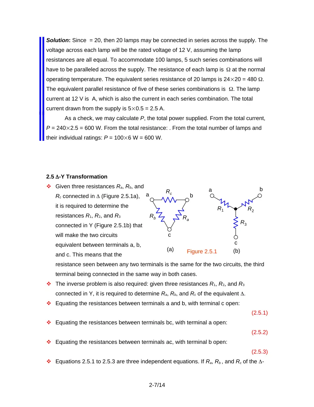2.5 -Y Transformation  Given three resistances Ra, Rb, and Rc connected in  (Figure 2.5.1a), it is required to determine the resistances R1, R2, and R3 connected in Y (Figure 2.5.1b) that will make the two circuits equivalent between terminals a, b, and c. This means that the resistance seen between any two terminals is the same for the two circuits, the third terminal being connected in the same way in both cases.  The inverse problem is also required: given three resistances R1, R2, and R3 connected in Y, it is required to determine Ra, Rb, and Rc of the equivalent .  Equating the resistances between terminals a and b, with terminal c open: (2.5.1)  Equating the resistances between terminals bc, with terminal a open: (2.5.2)  Equating the resistances between terminals ac, with terminal b open: (2.5.3)  Equations 2.5.1 to 2.5.3 are three independent equations. If Ra, Rb , and Rc of the - 2-7/14 Figure 2.5.1 Ra Rb Rc a b c c a b R1 R2 R3 (a) (b) circuit are given, these equations can be solved for R1, R2, and R3 of the equivalent Y-circuit: (2.5.4) (2.5.5) (2.5.6)  Conversely, if the resistances R1, R2 , and R3 of the Y-circuit are given, Equations 2.5.1 to 2.5.3 can be solved for Ra, Rb , and Rc of the equivalent -circuit: (2.5.7) (2.5.8) (2.5.9)  To help remember the above relations, the two equivalent circuits are superimposed (Figure 2.5.2). Each Y-resistance is the product of the -resistances on either side of it divided by the sum of the three -resistances. Conversely, each -resistance is the product of Y-resistances two at a time divided by the Y-resistance that is opposite the given -resistance. 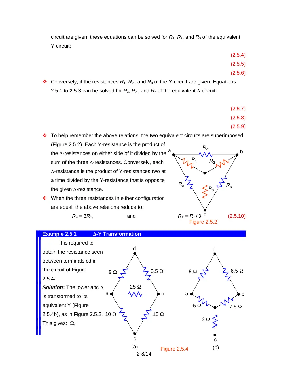 When the three resistances in either configuration are equal, the above relations reduce to: R = 3RY, and RY = R / 3 (2.5.10) Example 2.5.1 -Y Transformation It is required to obtain the resistance seen between terminals cd in the circuit of Figure 2.5.4a. Solution: The lower abc  is transformed to its equivalent Y (Figure 2.5.4b), as in Figure 2.5.2. This gives: , 2-8/14 Figure 2.5.4 a a b b c c d d 10  15  25  5  3  7.5  9  6.5  (a) (b) 9  6.5  c R1 R2 a b Rc Ra Rb Figure 2.5.2 R3 , and . The 5  resistance is then added to the 9  to give 14 , and the 7.5  resistance is added to the 6.5  to give 14 . The two 14  resistors in parallel give 7 , which is added to the 3  to give 10  between terminals cd. 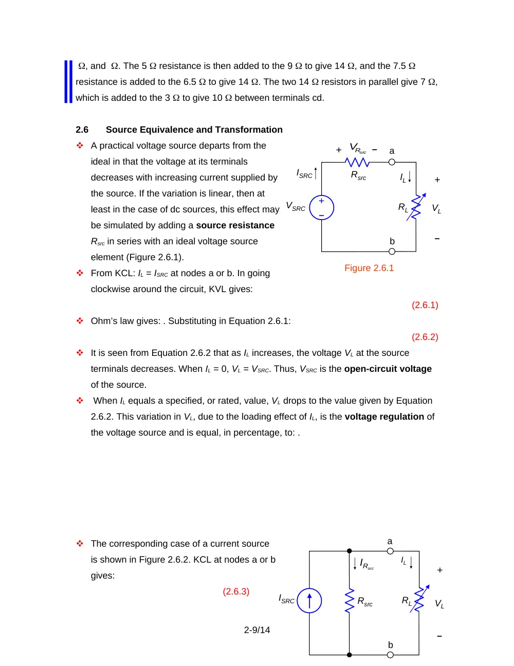2.6 Source Equivalence and Transformation  A practical voltage source departs from the ideal in that the voltage at its terminals decreases with increasing current supplied by the source. If the variation is linear, then at least in the case of dc sources, this effect may be simulated by adding a source resistance Rsrc in series with an ideal voltage source element (Figure 2.6.1).  From KCL: IL = ISRC at nodes a or b. In going clockwise around the circuit, KVL gives: (2.6.1)  Ohm’s law gives: . Substituting in Equation 2.6.1: (2.6.2)  It is seen from Equation 2.6.2 that as IL increases, the voltage VL at the source terminals decreases. When IL = 0, VL = VSRC. Thus, VSRC is the open-circuit voltage of the source.  When IL equals a specified, or rated, value, VL drops to the value given by Equation 2.6.2. This variation in VL, due to the loading effect of IL, is the voltage regulation of the voltage source and is equal, in percentage, to: .  The corresponding case of a current source is shown in Figure 2.6.2. KCL at nodes a or b gives: (2.6.3) 2-9/14 Rsrc VSRC + ISRC a b + IL VL RL Figure 2.6.1 – – – + Rsrc V ISRC Rsrc VL b a + IL RL – RI src  KVL is automatically satisfied since the same voltage VL is across all the circuit elements.  Multiplying both sides of Equation 2.6.3 by Rsrc and substituting : VL = RsrcISRC – RsrcIL (2.6.4)  When VL = 0, IL = ISRC. As VL increases, more of ISRC is diverted to Rsrc, so IL decreases. Current regulation occurs, analogous to voltage regulation in a voltage source. 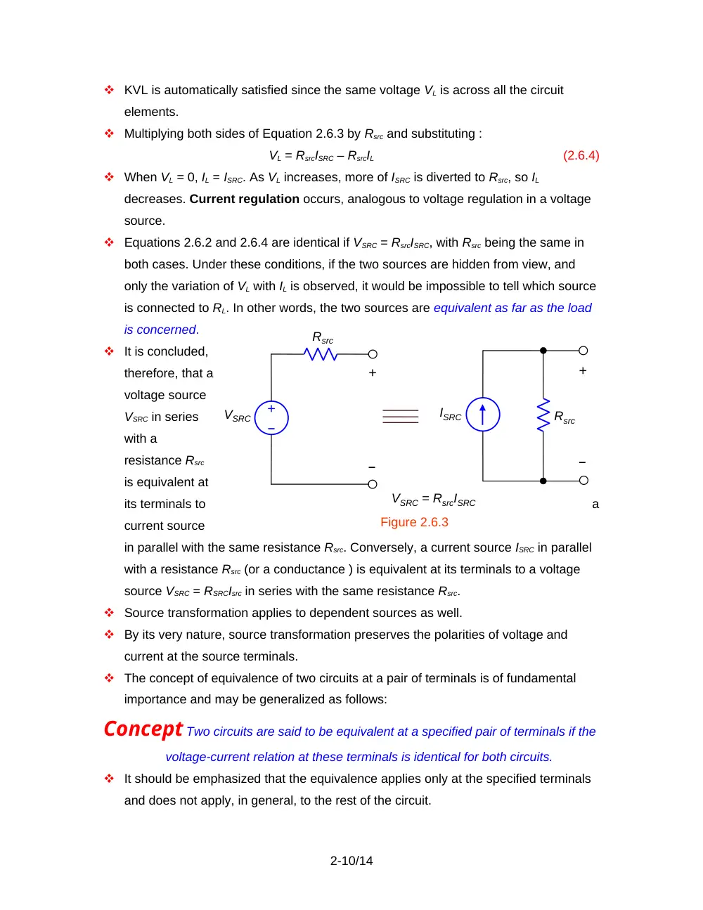 Equations 2.6.2 and 2.6.4 are identical if VSRC = RsrcISRC, with Rsrc being the same in both cases. Under these conditions, if the two sources are hidden from view, and only the variation of VL with IL is observed, it would be impossible to tell which source is connected to RL. In other words, the two sources are equivalent as far as the load is concerned.  It is concluded, therefore, that a voltage source VSRC in series with a resistance Rsrc is equivalent at its terminals to a current source in parallel with the same resistance Rsrc. Conversely, a current source ISRC in parallel with a resistance Rsrc (or a conductance ) is equivalent at its terminals to a voltage source VSRC = RSRCIsrc in series with the same resistance Rsrc.  Source transformation applies to dependent sources as well.  By its very nature, source transformation preserves the polarities of voltage and current at the source terminals.  The concept of equivalence of two circuits at a pair of terminals is of fundamental importance and may be generalized as follows: Concept Two circuits are said to be equivalent at a specified pair of terminals if the voltage-current relation at these terminals is identical for both circuits.  It should be emphasized that the equivalence applies only at the specified terminals and does not apply, in general, to the rest of the circuit. 2-10/14 VSRC Rsrc ISRC Figure 2.6.3 Rsrc – + VSRC = RsrcISRC + – + – Example 2.6.1 Equivalent Sources Given a voltage source having an open- circuit voltage of 12 V and a source resistance of 0.5  (Figure 2.6.4a). It is required to derive the equivalent current source. Solution: According to the above discussion, the equivalent current source has a source current of A and a source resistance of 0.5  (Figure 2.6.4b). If both sources are connected to a 5.5  load, for example, IL for the voltage source case is, from Figure 2.6.4 (a): IL = A, and VL = 25.5 = 11 V. In the case of the current source (Figure 2.6.4b), the resistance of the parallel combination is ; V, as in the case of the voltage source. However, the power delivered by the voltage source is whereas the power delivered by the current source is 1124 = 264 W. The power absorbed by Rsrc is W in the case of the voltage source and W in the case of the current source. Moreover, the current in the 0.5  resistor is not the same in both cases. It is 2A in (a) and 22 A in (b). Concept The ideal termination for a voltage source is an open circuit, whereas the ideal termination for a current source is a short circuit.  This is because the full voltage VSRC is available at the terminals of a voltage source only when IL = 0, that is, when the source terminals are open circuited. Similarly, the full current ISRC is available at the terminals of a current source only when VL = 0, that is, when the source terminals are short circuited. 2.7 Reduced-Voltage Supply  The simple resistive voltage divider is often used to supply a load at a reduced voltage.  The basic circuit is shown in Figure 2.7.1. 2-11/14 (a) 0.5  5.5  (b) 12 V IL 24 A IL Figure 2.6.4 – + + VL – 5.5  0.5  + VL – VSRC R1 + I1 + V1 I2 IL – + – Figure 2.7.2 SRC RV R R 2 1 2  R1||R2 – + + – VL Load Normally, VSRC is given together with the nominal load voltage VL and a range of variation of the load current IL. It is desired to determine R1 and R2 such that the variation in VL remains within specified limits as IL changes over the given range.  From KCL at either essential node: (2.7.1)  Applying KVL clockwise around the mesh composed of VSRC, R1, and R2: (2.7.2)  From Ohm’s law: and (2.7.3)  I1, I2 and V1 may be eliminated from the above four equations to give: (2.7.4) (2.7.5) where is the parallel resistance of R1 and R2.  Comparing Equation 2.7.5 with Equation 2.6.2, it follows that the voltage divider appears to the load as a source of open-circuit voltage , when IL = 0, and source resistance (Figure 2.7.2).  Given VSRC, VL, and IL, Equation 2.7.5 provides a relation between R1 and R2, but is not sufficient for uniquely determining their values. The additional information needed for this purpose comes from specifying the voltage variation VL = VL2 – VL1 forIL = IL2 – IL1. Substituting first VL1 and IL1, in Equation 2.7.5, then VL2 and IL2, and subtracting, eliminates the term in VSRC and gives: (2.7.6)  The interpretation of Equation 2.7.6 is that when is constant and IL changes by IL, VL is due to the voltage drop in, which is ()IL. The minus sign in Equation 2.7.6 signifies that VL decreases with IL.  It is desirable in practice to have a small VL for a given IL, which means that should be small. It is seen from Equation 2.7.5 that this makes small compared to the first term, , which means that . Under these conditions, is fixed for given VSRC and VL.  To reduce while keeping constant, both R1 and R2 should be reduced. But reducing 2-12/14 R1 and R2, increases the current drain from the supply, and generally increases the power dissipated in the voltage divider. This is undesirable, particularly in battery- operated equipment. Hence a tradeoff must be made in the design of the resistive voltage divider between good voltage regulation, that is, a small VL, on the one hand, and current drain from the supply and power dissipation in R1 and R2 on the other hand. For these reasons, the resistive voltage divider is impractical where there is a substantial variation in load current. Design Example 2.7.1 Voltage Regulation and Power Dissipation in a Voltage Divider A 3 V, 0.1 A dc load is to be supplied from a 12 V dc supply. The load current may vary by 20% of its nominal value of 0.1 A. The corresponding variation in the load voltage should not exceed 5% of the nominal value of 3 V. It is required to determine suitable values of R1 and R2. Solution: According to Equation 2.7.5, IL has its largest value when VL has its smallest value, and conversely. At IL = 0.80.1 = 0.08 A, VL = 1.053 = 3.15 V, and at IL = 1.20.1 = 0.12 A, VL = 0.953 = 2.85 V. Substituting these values in Equation 2.7.5 gives two relations between R1 and R2: , and From these, R1 = 24  and R2 =10.9 . Note that an easy way to solve these equations is to consider as one variable and as another variable. Let us calculate P, the total power dissipated in R1 and R2 under these conditions. With reference to Figure 2.7.1, . When VL = 3.15 V, P = 4.17 W, and when VL = 2.85 V, P = 4.23 W. P may not seem like an excessive amount of power. But if it is noted that the power consumed by the load does not exceed 0.34 W, when VL = 2.85 V and IL = 0.12 A, it is seen that of the power supplied by VSRC goes to the load under these conditions, the rest is dissipated in R1 and R2. The power efficiency is therefore quite poor. Suppose that in order to dissipate less power in R1 and R2, R1 is increased by a factor of 3 to 72 . From Equation 2.7.5: , which gives R2 = 120 . With these values of R1 and R2, VL = 3 V when IL = 0.1 A, and the power dissipated in R1 and R2 is now W. From Equation 2.7.6, –1.8 V. Thus, as IL changes from 0.08 A to 0.12 A, VL changes from V to V, a variation of 30% of the nominal value of 3 V. Such a variation will most likely not be acceptable. If the load current is constant, as may occur in the case of a lamp or a heater, for 2-13/14 example, R2 may be dispensed with altogether and only R1 used. If IL = 0.1 A and VL = 3 V, then  and the power dissipated is W. R1 is used in this case to drop the supply voltage by 9 V at 0.1 A. Design Example 2.7.2 Measurement of Partial Pressure of Oxygen The partial pressure of oxygen in the blood is measured as a direct indication of lung function, and as an indirect measurement of glucose concentration. Approximately 0.7 V is applied between two suitable electrodes, the resulting current being directly proportional to the partial pressure of oxygen in the solution. For the partial pressures normally of interest, the range of current is 0 to1.5 A. It is required to determine suitable values of R1 and R2, assuming VSRC = 12 V and VL = 0.7 V. Solution: A good guide for selecting R1, according to Equation 2.7.4, is to have the largest value of R1IL small compared to VSRC, say one-tenth of VSRC. Then, k. The nearest smaller standard value of a 5% tolerance resistor is 750 k. Using this value in Equation 2.7.5, with VL = 0.7 V and a mid-range value of IL = 0.75 A, gives R2 = 48.9 k. The nearest smaller standard value of a 5% tolerance resistor is 47 k. These values give VL = 0.708 V at IL = 0 and VL = 0.641 V at IL = 1.5 A. The variation in VL is about 5 % with respect to the nominal value of 0.7 V, which is quite acceptable. With R1||R2 = 44.23 k, the power dissipated in R1 and R2 is 0.18 mW, which is small because IL is small, so that R1 and R2 are relatively large. 2-14/14