EECE 210 Chapter 7, Fall 2012

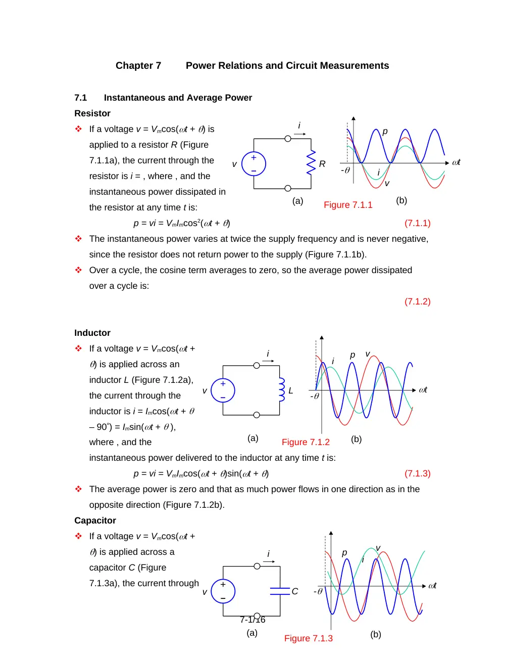
Chapter 7 Power Relations and Circuit Measurements 7.1 Instantaneous and Average Power Resistor  If a voltage v = Vmcos(t + ) is applied to a resistor R (Figure 7.1.1a), the current through the resistor is i = , where , and the instantaneous power dissipated in the resistor at any time t is: p = vi = VmImcos2(t + ) (7.1.1)  The instantaneous power varies at twice the supply frequency and is never negative, since the resistor does not return power to the supply (Figure 7.1.1b).  Over a cycle, the cosine term averages to zero, so the average power dissipated over a cycle is: (7.1.2) Inductor  If a voltage v = Vmcos(t + ) is applied across an inductor L (Figure 7.1.2a), the current through the inductor is i = Imcos(t +  – 90) = Imsin(t +  ), where , and the instantaneous power delivered to the inductor at any time t is: p = vi = VmImcos(t + )sin(t + ) (7.1.3)  The average power is zero and that as much power flows in one direction as in the opposite direction (Figure 7.1.2b). Capacitor  If a voltage v = Vmcos(t + ) is applied across a capacitor C (Figure 7.1.3a), the current through 7-1/16 v R i (a) (b) Figure 7.1.1 p v i - t – + t L i (a) (b) p v i - v – + Figure 7.1.2 C (a) (b) p v i - t v – + i Figure 7.1.3 the capacitor is i = Imcos(t +  + 90) = -Imsin(t + ), where , and the instantaneous power delivered to the capacitor at any time t is: p = vi = -VmImcos(t + )sin(t + ) (7.1.4)  The average power is zero and as much power flows in one direction as in the opposite direction (Figure 7.1.3b). Concept When v and i are sinusoidal functions of time of frequency , with v being a voltage drop in the direction of i, the instantaneous power p = vi is pulsating at a frequency 2. If v is in phase with i, as in the case of R, p  0 and represents power dissipated. If v and i are in phase quadrature, as in the case of L and C, p is purely alternating, of zero average, since no power is dissipated. In this case, when v and i have the same sign, p > 0 and represents energy being stored in the energy-storage element. When v and i have opposite signs, p < 0 and represents previously stored energy being returned to the rest of the circuit. 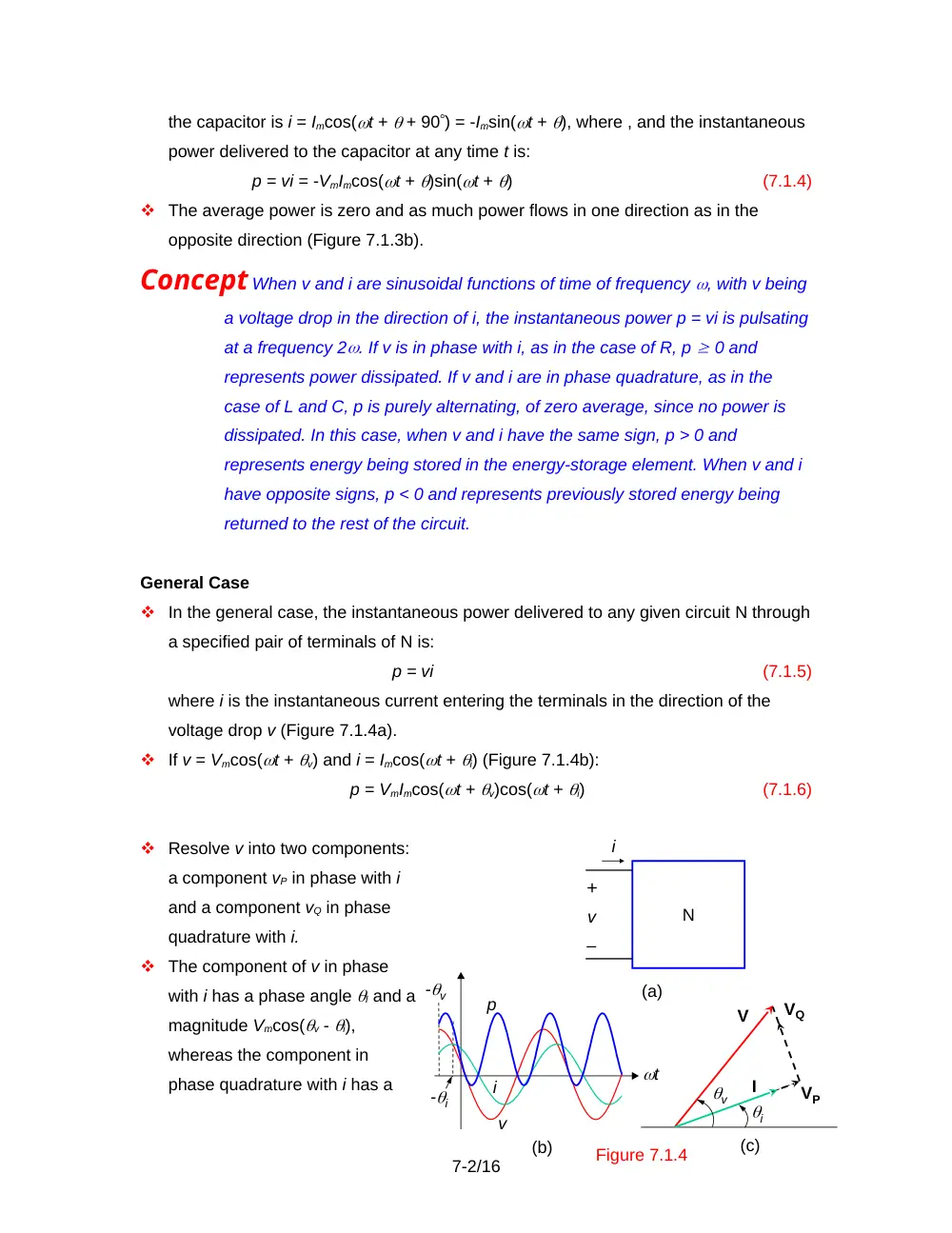General Case  In the general case, the instantaneous power delivered to any given circuit N through a specified pair of terminals of N is: p = vi (7.1.5) where i is the instantaneous current entering the terminals in the direction of the voltage drop v (Figure 7.1.4a).  If v = Vmcos(t + v) and i = Imcos(t + i) (Figure 7.1.4b): p = VmImcos(t + v)cos(t + i) (7.1.6)  Resolve v into two components: a component vP in phase with i and a component vQ in phase quadrature with i.  The component of v in phase with i has a phase angle I and a magnitude Vmcos(v - i), whereas the component in phase quadrature with i has a 7-2/16 -v (a) (b) N i – + v p v i -i t (c) i v I VP V VQ Figure 7.1.4 phase angle (I + 90) and a magnitude Vmsin(v - i) (Figure 7.1.4c). Thus: vP = [Vmcos(v - i)]cos(t + i)] (7.1.7) vQ = Vmsin(v - i)cos(t + i + 90) = –Vmsin(v – i)sin(t + i) (7.1.8)  Multiplying each of the two components of v by i: vPi = VmImcos(v – i)cos2(t + i) = P[1 + cos2(t + i)] (7.1.9) where, (7.1.10) and vQi = –VmImsin(v - i)cos(t + i)sin(t + i) = Qcos[2(t + i) + 90] (7.1.11) where, (7.1.12)  P is the real, or average, power. It appears in Equation 7.1.9 both as the average of vPi, which is the power dissipated in the resistive elements of the circuit, and as the magnitude of the alternating component of vPi.  Q is the reactive power and is the power associated with the energy that is alternately stored and returned to the supply by the inductive and capacitive elements of the circuit. From Equation 7.1.12, Q is the magnitude of vQi, which is purely alternating.  For a resistor, , so Q = 0 and P = VrmsIrms, in accordance with Equation 7.1.2. For an inductor, , so Q = VrmsIrms and P = 0. For a capacitor, , so Q = –VrmsIrms and P = 0. Thus, Q is positive for an inductive reactance and is negative for a capacitive reactance.  Whereas the unit of P is the watt (W), the unit of Q is the volt-ampere reactive, VAR). 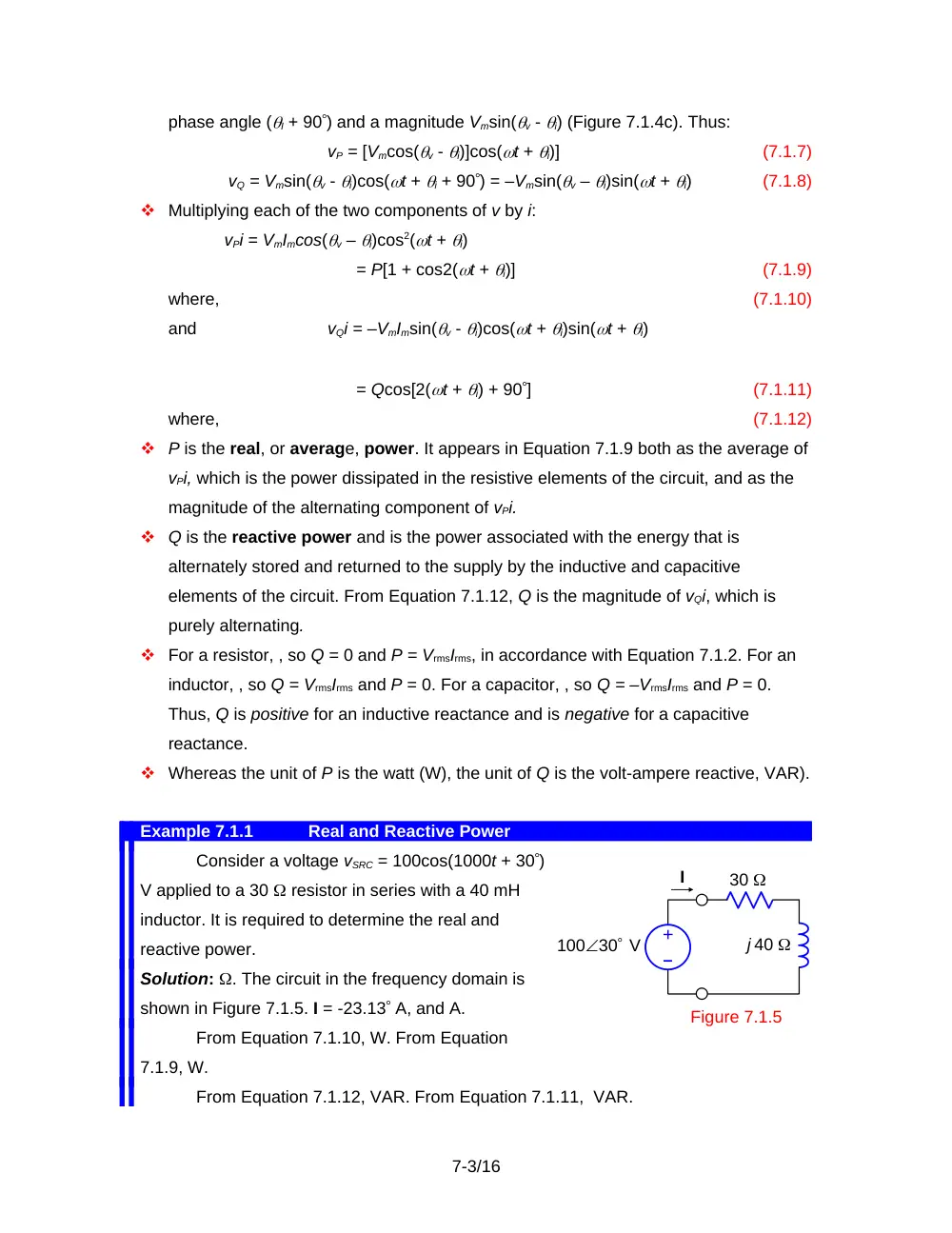Example 7.1.1 Real and Reactive Power Consider a voltage vSRC = 100cos(1000t + 30) V applied to a 30  resistor in series with a 40 mH inductor. It is required to determine the real and reactive power. Solution: . The circuit in the frequency domain is shown in Figure 7.1.5. I = -23.13 A, and A. From Equation 7.1.10, W. From Equation 7.1.9, W. From Equation 7.1.12, VAR. From Equation 7.1.11, VAR. 7-3/16 I – + Figure 7.1.5 30  j 40  10030 V P is the average power dissipated in the resistor, which is also = W. The maximum instantaneous power dissipation is 2P = 120 W and occurs when . The energy stored in the inductor at any instant is . The rate at which this energy is stored is = , which is the same as Equation 7.1.11, where VAR. 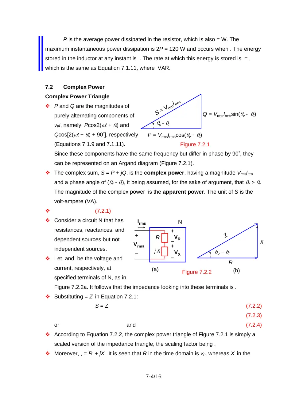7.2 Complex Power Complex Power Triangle  P and Q are the magnitudes of purely alternating components of vPi, namely, Pcos2(t + i) and Qcos[2(t + i) + 90], respectively (Equations 7.1.9 and 7.1.11). Since these components have the same frequency but differ in phase by 90, they can be represented on an Argand diagram (Figure 7.2.1).  The complex sum, S = P + jQ, is the complex power, having a magnitude VrmsIrms and a phase angle of (v - i), it being assumed, for the sake of argument, that v > i. The magnitude of the complex power is the apparent power. The unit of S is the volt-ampere (VA).  (7.2.1)  Consider a circuit N that has resistances, reactances, and dependent sources but not independent sources.  Let and be the voltage and current, respectively, at specified terminals of N, as in Figure 7.2.2a. It follows that the impedance looking into these terminals is .  Substituting = Z in Equation 7.2.1: S = Z (7.2.2) (7.2.3) or and (7.2.4)  According to Equation 7.2.2, the complex power triangle of Figure 7.2.1 is simply a scaled version of the impedance triangle, the scaling factor being .  Moreover, , = R + jX . It is seen that R in the time domain is vP, whereas X in the 7-4/16 Figure 7.2.1 P = VrmsIrmscos(v  i) Q = VrmsIrmssin(v  i) S = VrmsIrms v - i (a) (b) Figure 7.2.2 – + Irms Vrms N R j X + + – –VR VX Z X R v – i time domain is vQ. 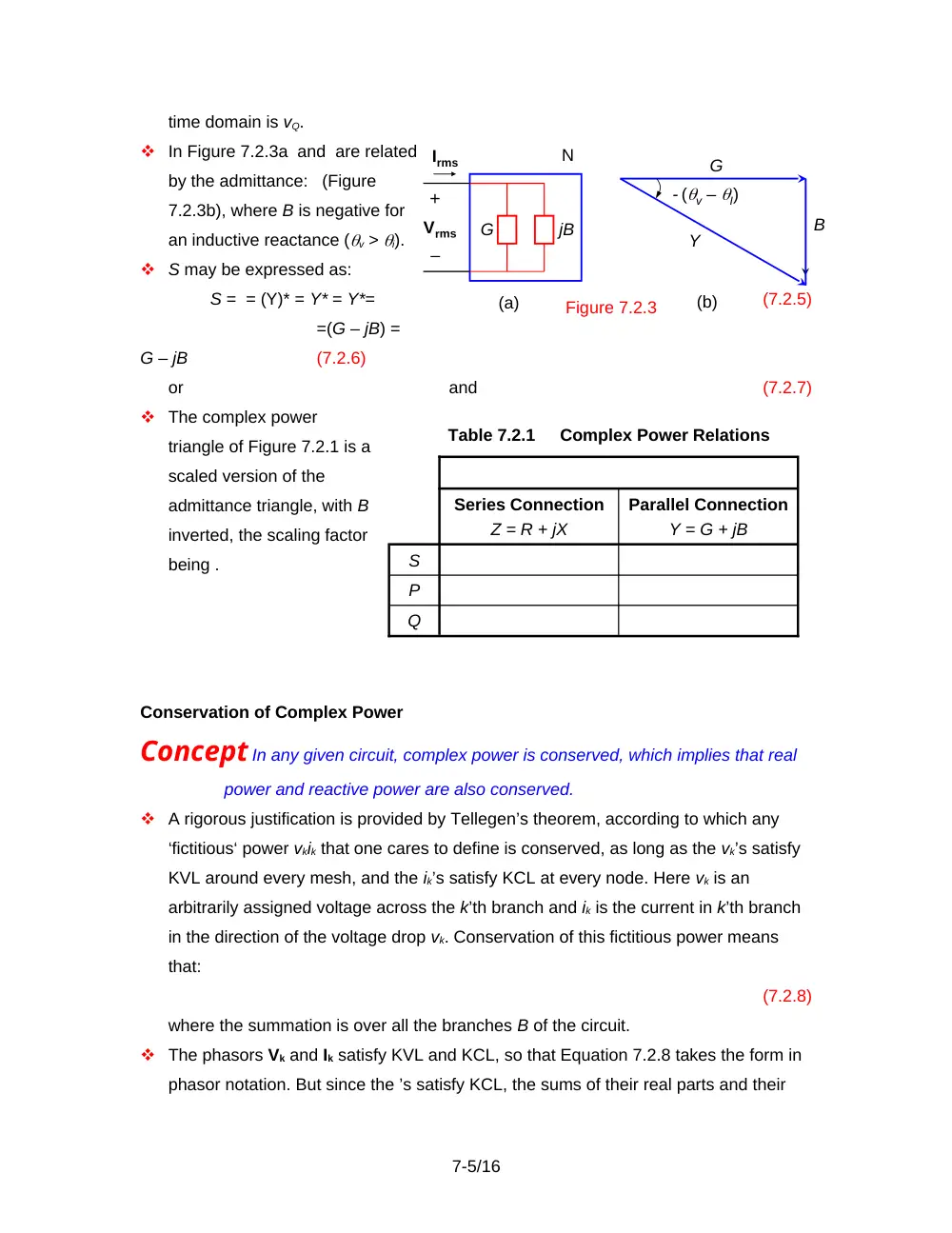 In Figure 7.2.3a and are related by the admittance: (Figure 7.2.3b), where B is negative for an inductive reactance (v > i).  S may be expressed as: S = = (Y)* = Y* = Y*= (7.2.5) =(G – jB) = G – jB (7.2.6) or and (7.2.7)  The complex power triangle of Figure 7.2.1 is a scaled version of the admittance triangle, with B inverted, the scaling factor being . Conservation of Complex Power Concept In any given circuit, complex power is conserved, which implies that real power and reactive power are also conserved.  A rigorous justification is provided by Tellegen’s theorem, according to which any ‘fictitious‘ power vkik that one cares to define is conserved, as long as the vk’s satisfy KVL around every mesh, and the ik’s satisfy KCL at every node. Here vk is an arbitrarily assigned voltage across the k’th branch and ik is the current in k’th branch in the direction of the voltage drop vk. Conservation of this fictitious power means that: (7.2.8) where the summation is over all the branches B of the circuit.  The phasors Vk and Ik satisfy KVL and KCL, so that Equation 7.2.8 takes the form in phasor notation. But since the ’s satisfy KCL, the sums of their real parts and their 7-5/16 – + Vrms B (a) Irms N G jB G (b) Y - (v – I) Figure 7.2.3 Table 7.2.1 Complex Power Relations Series Connection Z = R + jX Parallel Connection Y = G + jB S P Q imaginary parts are each separately equal to zero. It follows that the ’s also satisfy KCL. Hence: (7.2.9)  Equation 7.2.9 is an expression of the conservation of complex power. Moreover, since Sk = Pk + jQk, it follows that Pk and Qk must each sum to zero: and (7.2.10)  In making these summations, real power is considered positive if dissipated and negative if delivered. Inductive power is considered positive if absorbed and negative if delivered. Conversely, capacitive power is considered negative if absorbed and positive if delivered. Concept Real power and reactive power can each be summed branch by branch in a given circuit, with the total sum of each, over all branches of the circuit, equal to zero. 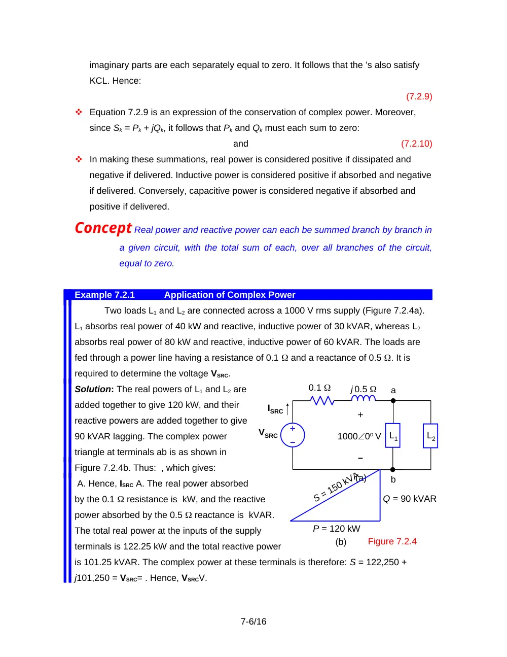Example 7.2.1 Application of Complex Power Two loads L1 and L2 are connected across a 1000 V rms supply (Figure 7.2.4a). L1 absorbs real power of 40 kW and reactive, inductive power of 30 kVAR, whereas L2 absorbs real power of 80 kW and reactive, inductive power of 60 kVAR. The loads are fed through a power line having a resistance of 0.1  and a reactance of 0.5 . It is required to determine the voltage VSRC. Solution: The real powers of L1 and L2 are added together to give 120 kW, and their reactive powers are added together to give 90 kVAR lagging. The complex power triangle at terminals ab is as shown in Figure 7.2.4b. Thus: , which gives: A. Hence, ISRC A. The real power absorbed by the 0.1  resistance is kW, and the reactive power absorbed by the 0.5  reactance is kVAR. The total real power at the inputs of the supply terminals is 122.25 kW and the total reactive power is 101.25 kVAR. The complex power at these terminals is therefore: S = 122,250 + j101,250 = VSRC= . Hence, VSRCV. 7-6/16 (a) j 0.5  VSRC b 0.1  a + – 10000o V ISRC – + L1 L2 Figure 7.2.4 (b) S = 150 kVA P = 120 kW Q = 90 kVAR The real power delivered by the source is 122.25 kW. It is the sum of the real power dissipated in the line resistance and in loads L1 and L2. The reactive power delivered by the source is 101.25 kVAR. It is also the sum of the inductive reactive power in the line reactance and in the two loads. Real and reactive power are conserved in the system as a whole. 7.3 Power Factor Correction Concept Reactive power, although it averages to zero over a cycle, generally increases the voltage and current requirements of a load.  In Figure 7.2.2a, the real power delivered to the load is . To deliver a given Irms in the presence of the reactance X requires a larger voltage across the series combination, and therefore a higher degree of insulation of the conductors subjected to the higher voltage.  Similarly, in Figure 7.2.3a, the real power delivered to the load is . To apply a given Vrms in the presence of the susceptance B requires a larger current through the parallel combination, and therefore a greater current-carrying capacity of the supply conductors.  The relative value of the reactive component of a load is indicated by the phase angle (v – i); cos(v – i) is the power factor (abbreviated p.f.), and sin(v – i) is the reactive factor. For a purely resistive load, the p.f. is unity.  Since the p.f. is the same for a positive (v – i) as for a negative (v – i), these two cases are distinguished by adding the attribute ‘lagging’ or ‘leading’, respectively. For example, for a purely inductive load, v – i = 90, and the p.f. is zero lagging, whereas for a purely capacitive load, v – i = –90, and the p.f. is zero leading.  A low p.f. is undesirable because of the additional current and voltage burdens placed on the supply. In the case of large loads, the additional costs involved can be quite considerable, so that some measures are taken to improve the power factor. This power factor correction is achieved by adding capacitive reactance to counteract the inductive reactance of the load. Example 7.3.1 Power Factor Correction Assuming the supply frequency is 50 Hz, determine the capacitance that must be added in parallel with the loads of Figure 7.2.4 of Example 7.2.1 so as to make the p.f. 7-7/16 unity at terminals ab. What is the effect of this capacitance on the supply current and voltage? Solution: The reactive power at terminals ab was found in Example 7.2.1 to be 90 kVAR. The reactive power of the added capacitor must be –90 kVAR. The value of capacitance follows from the fact 2fCV2 = – Q (Equation 7.2.6). Thus, , or C = 286.5 F. The total reactive power at terminals ab is now zero. Hence, S = 120,000 = . This gives: = 1200 A. The real power absorbed by the 0.1  resistance is kW, and the reactive power absorbed by the 0.5  reactance is kVAR. The total real power at the inputs of the supply terminals is 121.44 kW and the total reactive power is 7.2 kVAR. The complex power at these terminals is therefore: VSRC . Hence, VSRC V. The p.f. at the load was initially = 0.8. By correcting it to 1 the supply current was reduced from 150 A to 120 A and the supply voltage was reduced by a relatively small amount in this case, from 1058 to 1014 V rms, due to the reduced voltage drop across the line impedance. 7.4 Maximum Power Transfer  A matter of practical importance is to transfer maximum power to a load from a given source of specified open-circuit voltage and source impedance. Purely Resistive Circuit  In Figure 7.4.1, , and the power transferred to is: (7.4.1)  With VSRC and Rsrc constant, we wish to find the value of that maximizes If we derive and set it to zero, we find that is maximum for given by: (7.4.2)  When Equation 7.4.2 is satisfied, the source and load resistances are matched. 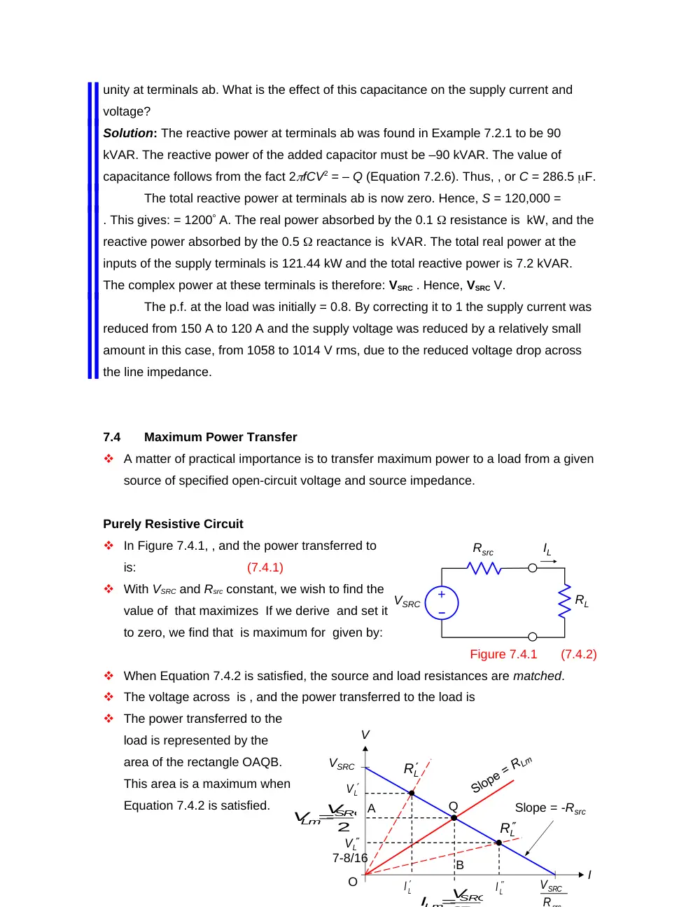 The voltage across is , and the power transferred to the load is  The power transferred to the load is represented by the area of the rectangle OAQB. This area is a maximum when Equation 7.4.2 is satisfied. 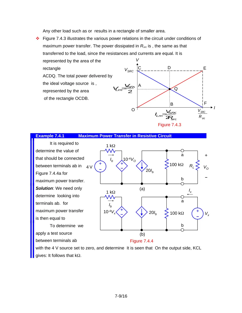7-8/16 Rsrc RL VSRC IL – + Figure 7.4.1 V VSRC Q O Slope = -Rsrc I L V  LI  L V  L R L R  2 SRC Lm V V  src SRC R V SRC ILm V  A B LI  Figure 7.4.3 V VSRC Q O I 2 SRC Lm V V  src SRC R V src SRC Lm R V I 2  A B C D E F Any other load such as or results in a rectangle of smaller area.  Figure 7.4.3 illustrates the various power relations in the circuit under conditions of maximum power transfer. The power dissipated in Rsrc is , the same as that transferred to the load, since the resistances and currents are equal. It is represented by the area of the rectangle ACDQ. The total power delivered by the ideal voltage source is , represented by the area of the rectangle OCDB. Example 7.4.1 Maximum Power Transfer in Resistive Circuit It is required to determine the value of that should be connected between terminals ab in Figure 7.4.4a for maximum power transfer. Solution: We need only determine looking into terminals ab. for maximum power transfer is then equal to To determine we apply a test source between terminals ab with the 4 V source set to zero, and determine It is seen that On the output side, KCL gives: It follows that k. 7-9/16 4 V – + 20Ib 10-4VO 1 k + – VO a b 100 k (a) Figure 7.4.4 Ib + – RL (b) 20Ib 10-4Vx 1 k + – Vx a b 100 k Ib + – Ix Source and Load Impedances  Let VSRC and Zsrc = Rsrc + jXsrc represent, in general, the TEC as seen from terminals ab of a given circuit connected to a load ZL = RL +jXL. The current phasor IL is given by: ILVSRC (7.4.5)  Assuming that IL is expressed in terms of its rms value, the power transferred to RL is: (7.4.6)  If RL and XL can be varied independently, it is clear that, with RL fixed, PL is maximum for XL given by: XLm = –Xsrc (7.4.7)  With this condition satisfied, Equation 7.4.6 reduces to Equation 7.4.1. PL is maximum when Equation 7.4.2 is satisfied, that is, RLm = Rsrc.  Combining this condition with that of Equation 7.4.7, gives the condition for maximum power transfer as: (7.4.8) where is the conjugate of Zsrc.  If RL and XL can be varied independently, but their range of variation is restricted, it is clear from Equation 7.4.6 that under these conditions, with RL fixed, PL is maximum when (Xsrc + XL) is as small as possible. With (Xsrc + XL) considered constant, the condition for maximum power transfer can be determined by deriving from Equation 7.4.6 and setting it to zero. This gives: (7.4.9)  If RL cannot be made equal to this value, then a value of RL as close to it as possible will give maximum power transfer.  Another case of interest arises from the use of a transformer with ZL. The load impedance reflected to the primary side is ideally , where Np and Ns are the number of turns of the primary and secondary windings, respectively. It follows that . The effect of an ideal transformer is to vary while the phase angle remains constant.  To derive the condition for maximum power transfer under these conditions, we substitute in Equation 7.4.6 , , , and to obtain: (7.4.10) 7-10/16 Figure 7.4.9 j 2  1:5 1400 V rms jXL b 2  6  a RL – + where the only variable on the RHS is .  Deriving and setting it equal to zero gives for the condition of maximum power transfer: (7.4.11) Example 7.4.2 Maximum Power Transfer with Variable Load Impedance Given the circuit of Figure 7.4.9, it is required to determine the condition for maximum power transfer, and the power transferred to RL, under the following conditions: (a) Both RL and XL are variable independently. (b) RL is fixed at 35  and XL is variable. (c) XL is fixed at –50  and RL is variable. (d) RL is fixed at 35 , XL is fixed at –50 , and the transformer can be selected to have any desired ratio. Solution: The first step is to derive TEC looking into terminals ab towards the source, and reflect TEC to the secondary side. When terminals ab are open-circuited, V rms. With the source set to zero, the impedance looking into terminals ab is ZTh = 6 + 7 + j . Reflecting TEC to the secondary side, it becomes a voltage source of 70(1 + j)5 = 350(1 + j) V rms in series with (7 + j)25 = 175 + j25  (Figure 7.4.10). 7-11/16  45 2 350 V jX L 175  RL j 25  – + Figure 7.4.10 rms Table 7.4.1 Conditions for Maximum Power Transfer Allowed Variation Condition for Maximum Power Transfer RL and XL can be varied independently over an arbitrary range RLm = Rsrc and XLm = -Xsrc RL is fixed but XL can be varied XLm = -Xsrc XL is fixed but RL can be varied RL and XL can be varied independently over a restricted range XLm as close to -Xsrc as possible, RLm as close to as possible. can be varied, while L is constant (a) If both RL and XL can be varied independently, the condition for maximum power transfer is given by Equation 7.4.8: RLm = 175  and XLm = –25 . The power transferred to RLm is W. (b) If RL = 35  and XL is variable, maximum power transfer occurs when XLm = –25 as in (a). The power transferred to RL is W. (c) If XL = – 50  and RL is variable, the condition for maximum power transfer is given by Equation 7.4.9: = 176.8 . The magnitude of the current is A rms, and the power transferred to RLm is W. (d) If RL is fixed at 35  and XL is fixed at -50 , 61.0 . The magnitude of ZTh is . The turns ratio, instead of 1:5 should be , or 1:2.94, which is nearly 1:3. TEC reflected to the secondary side will be a source of magnitude V rms in series with a resistance of  and a reactance of . The magnitude of the current is 2.8 A rms, and the power transferred to RL is W. Admittance Relations  Let ISRC and Ysrc represent, in general, NEC as seen from terminals ab of a given circuit connected to a load YL = GL + jBL. The corresponding relations to Equations 7.4.8, 7.4.9, and 7.4.11 are, respectively: (7.4.12) (7.4.13) (7.4.14) Example 7.4.3 Admittance Power Relations Given the circuit of Figure 7.4.12. It is required to determine the condition for maximum power transfer, and the power transferred to RL, assuming that: (a) Both RL and X are variable independently. (b) Both RL and X are variable independently 7-12/16 Figure 7.4.12 – + 10  j 10  30 0o V Rsrc j Xsrc j 20  j X RL but only over the magnitude range 30 to 50  each. (c) If RL is fixed at 30  and X is variable, what is the condition for minimum power dissipated in Rsrc and how much is this power? Solution: (a) Let us convert the source and its impedance to its NEC. The Norton source current is: A rms. The Norton admittance is: S. The circuit becomes as shown in Figure 7.4.13. According to Equation 7.4.12, maximum power is transferred to the load when Bm = -BN and GLm = GN. The first condition gives: , from which: Xm = -10 . The second condition gives: , or RL = 20 . Under these conditions, the current in GL is , and the power transferred to GL is W. (b) If X is variable between -30 and -50 , B is variable between and S. Maximum power transfer occurs when B has its largest positive value, which is . Under these conditions the total susceptance is . GLm for maximum power transfer is then given by Equation 7.4.13 as: S. The value of GL nearest to this is S. Maximum power is transferred under these conditions when RL and X have a magnitude of 30  each. To find the maximum power transferred, we note that the circuit reduces under these conditions to that shown in Figure 7.4.14. The admittance Yx of the combination is . The voltage VxIN, so, |Vx||IN| and the power transferred to GL is: GL|Vx|2 W. (c) If RL is fixed and X is variable, minimum power is dissipated in Rsrc when the current in this resistor is a minimum. With the source reactance fixed, the current in Rsrc is a minimum when the impedance of the parallel combination of the load in Figure 7.4.12 is a maximum, that is, when the admittance YL is a minimum. , or S. With X the only variable in this relation, is a minimum when the second bracketed term, vanishes, that is when X = -20. The circuit 7-13/16 + – Vx S 30 1 A 245 5 . 1  o  S 20 1 A 15 j  Figure 7.4.14 30  – + 10  j 10  I 300o V Figure 7.4.15 GL X j  S 20  j S 20 1 A 245 5 . 1  o  S 20 j  Figure 7.4.13 reduces to that of Figure 7.4.15. The current I, and |I| A. The power dissipated in Rsrc is Rsrc|I|2 W. 7.5 Measurement of Current, Voltage, and Power  The older measuring instruments are analog, the deflection of the indicating pointer being proportional (or analogous) to the current passing through the instrument. Modern instruments are digital; the quantity to be measured is sampled, digitized, and displayed as numerical digits.  Compared to analog instruments, digital instruments are more accurate, generally have negligible loading effects, can measure very low values of current or voltage, and can change ranges automatically. Nevertheless, analog instruments are useful for quick monitoring of the quantity being measured and for quick verification of normal or safe levels.  A basic type of analog movement, the moving coil or D’Arsonval movement, consists essentially of a current-carrying coil that is free to rotate in the magnetic field of a permanent magnet (Figure 7.5.1). A pointer attached to the coil can move relative to a calibrated scale.  With proper design, the angle of rotation is directly proportional to the coil current, resulting in a linear scale.  In order to measure the current passing through a given circuit element, an ammeter is connected in series with the element (Figure 7.5.2).  An ideal ammeter has zero impedance, so that it does not introduce additional impedance in series with Z, which would affect the current being measured. For example, if the circuit in Figure 7.5.2 has a TEC between terminals ab of 50 V in series with a 25  resistance and that Z also equals 25 . The current in the circuit is then 1 A. If an ammeter of 1  resistance is used to measure the current, the total resistance in the circuit becomes 51 , and the ammeter reading will be A, which is in error by nearly -2%. 7-14/16 Circuit Z A a b Figure 7.5.2 N S Figure 7.5.1 Calibrated scale Current-carrying coil 0 10  In order to measure the voltage across a given circuit element, a voltmeter is connected in parallel with the element, (Figure 7.5.3).  An ideal voltmeter should have infinite impedance, so that it does not introduce additional impedance in parallel with Z, which would affect the voltage being measured. For example, if we assume that the circuit in Figure 7.5.3 has an NEC between terminals ab of 1A in parallel with a 50  resistance and that Z also equals 50 . It follows that Vab = 25 V. If a voltmeter of 2.5 k is used to measure the voltage, the total resistance becomes 25||2,500 = 24.75 . The voltmeter reading will be 24.75 V, which is in error by nearly -1%. Concept For accurate current and voltage measurements, the impedance of an ammeter should be small compared with the impedance that appears in series with it, and the impedance of a voltmeter should be large compared with the impedance that appears in parallel with it. Power Measurements  Since , the apparent power |S| at any location is determined by measuring and at that location by means of an ac voltmeter and an ac ammeter, respectively.  To measure the real power, a wattmeter is used. The wattmeter has two coils, a current coil and a voltage coil with polarity markings. The current coil is connected like an ammeter so that the load current flows through it. The voltage coil is connected across the load terminals, like a voltmeter. 7-15/16 Circuit Z V Figure 7.5.3 a b Current coil Load + – V I + + – – Voltage coil Figure 7.5.4  When the polarities of the two coils with respect to I and V are as indicated in Figure 7.5.4, the wattmeter reads the power absorbed, . If the polarity of either coil is reversed, the wattmeter gives a negative indication.  Knowing P and , Q and the p.f. readily follow from the complex power triangle. 7-16/16