EECE 210 Chapter Uploading Chapter 08 Sinusoidal Steady, Spring 2015

Chapter 8 Sinusoidal Steady State The present chapter is concerned with introducing a special methodology for the analysis of a circuit excited by sinusoidal functions of time in the steady state. The methodology is based on expressing voltages and currents as phasors and the voltage-current relation of circuit elements in terms of impedance. Linear differential equations describing the behavior of circuits involving capacitors and inductors are thereby reduced to algebraic equations involving the imaginary unit j. This greatly simplifies circuit analysis and extends to the sinusoidal steady state all the concepts, theorems, and procedures applied to resistive circuits under dc conditions, in addition to other advantages mentioned in Section 8.1. The chapter is therefore mainly concerned with developing the concepts of phasors and impedance and applying them in several illustrative examples. 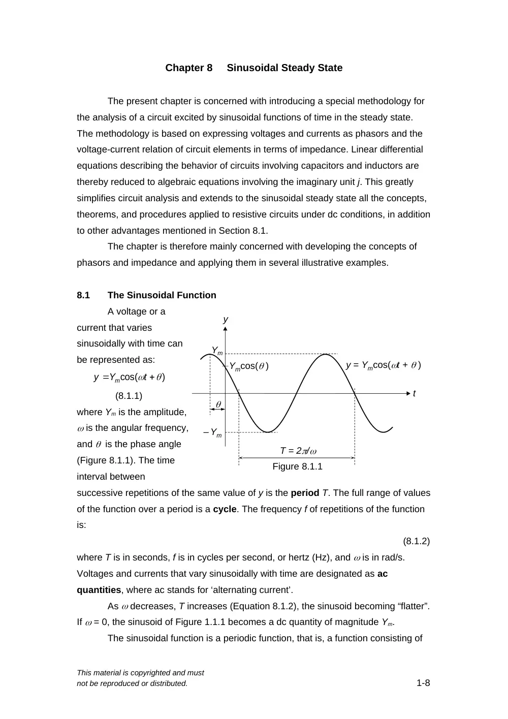8.1 The Sinusoidal Function A voltage or a current that varies sinusoidally with time can be represented as: (8.1.1) where Ym is the amplitude,  is the angular frequency, and  is the phase angle (Figure 8.1.1). The time interval between successive repetitions of the same value of y is the period T. The full range of values of the function over a period is a cycle. The frequency f of repetitions of the function is: (8.1.2) where T is in seconds, f is in cycles per second, or hertz (Hz), and  is in rad/s. Voltages and currents that vary sinusoidally with time are designated as ac quantities, where ac stands for ‘alternating current’. As  decreases, T increases (Equation 8.1.2), the sinusoid becoming “flatter”. If  = 0, the sinusoid of Figure 1.1.1 becomes a dc quantity of magnitude Ym. The sinusoidal function is a periodic function, that is, a function consisting of This material is copyrighted and must not be reproduced or distributed. 1-8 y Ym T = 2/ Ymcos( ) Figure 8.1.1 – Ym t y = Ymcos(t +  )  ) cos(    t Y y m cycles that repeat at a given frequency. However, it is the only periodic function that has only a single frequency. In fact, according to Fourier’s theorem (Chapter 16), a periodic function can generally be considered as the sum of a theoretically infinite number of cosine and sine functions whose frequencies are integral multiples of the frequency of the periodic function. An important implication of this characteristic of sinusoidal functions is: Concept: When a sinusoidal excitation is applied to an LTI circuit, all the currents and voltages in the circuit are sinusoidal functions, generally having different amplitudes and phase angles, but all having the same frequency as the excitation. The reason for this is that voltages and currents in an LTI circuit are subject to linear operations such as: i) scaling, or multiplication by a constant, as in voltage or current division, ii) addition and subtraction, as in KCL or KVL, and iii) differentiation and integration, as in the v-i relations of inductors and capacitors. When sinusoidal functions are subjected to any of these linear operations, they remain sinusoidal functions of the same frequency. The amplitudes and phase angles of the resulting sinusoidal functions will differ from those of the original functions, but no new frequencies are produced. Another important property of the sinusoidal function, which is used in this chapter, is embodied in De Moivre’s theorem: (8.1.3) where j = is the imaginary unit and Ym is the amplitude of the sinusoidal function. is a complex quantity, whose real component is Ymcost and whose imaginary component is jYmsint. The term Ymsint, without j, is the imaginary part. The real part and the real component are, of course, one and the same. 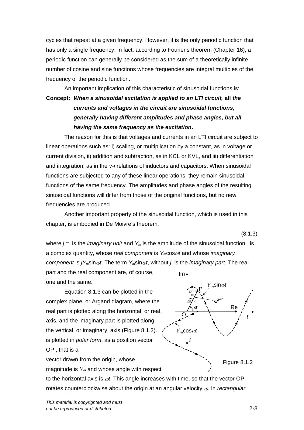Equation 8.1.3 can be plotted in the complex plane, or Argand diagram, where the real part is plotted along the horizontal, or real, axis, and the imaginary part is plotted along the vertical, or imaginary, axis (Figure 8.1.2). is plotted in polar form, as a position vector OP , that is a vector drawn from the origin, whose magnitude is Ym and whose angle with respect to the horizontal axis is t. This angle increases with time, so that the vector OP rotates counterclockwise about the origin at an angular velocity . In rectangular This material is copyrighted and must not be reproduced or distributed. 2-8 Figure 8.1.2 Im Re P Ym  t t t Ymsint Ymcost O t je  form, Ymcost is the projection of along the real axis, and Ymsint is its projection on the imaginary axis. As time progresses, the lengths of these projections vary sinusoidally with time, as illustrated by the dashed extensions in Figure 8.1.2. Analysis of the sinusoidal steady state is the derivation of the currents and voltages in a circuit after a sinusoidal excitation has been applied for a sufficiently long time. When any excitation is suddenly applied to a circuit, there is generally an initial “transient”, or temporary, response that dies out with time, as explained in later chapters. After this transient dies out, a steady-state remains, in which the currents and voltages repeat according to some pattern that depends on the time variation of the excitation. Analysis of the sinusoidal steady state is of fundamental importance for the following reasons: 1. The sinusoidal steady state is used in several practical cases, as in the frequency response of systems (Chapter 14) and in power systems analysis (Chapter 25). Electric power is efficiently generated, transmitted, and distributed as sinusoidal voltages. 2. The methodology used in steady state sinusoidal analysis is based on expressing sinusoidal voltages and currents as phasors and the v-i relations in terms of impedance. This is extremely convenient in that it extends to the sinusoidal steady state all the concepts, theorems, and procedures that apply to resistive circuits under dc conditions. 3. This representation of sinusoidal voltages and currents as phasors and the v-i relations in terms of impedance are later applied to the analysis of frequency responses of circuits (Chapter 14), the responses to periodic inputs (Chapter 16), complex power and three-phase systems (Chapter 25), and the Fourier transform (Chapter 22). Moreover, the same representation can be readily generalized to the most powerful method for analyzing linear systems, namely that of the Laplace transform (Chapter 21). 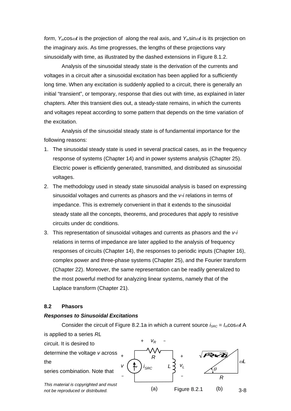8.2 Phasors Responses to Sinusoidal Excitations Consider the circuit of Figure 8.2.1a in which a current source iSRC = Imcost A is applied to a series RL circuit. It is desired to determine the voltage v across the series combination. Note that This material is copyrighted and must not be reproduced or distributed. 3-8 R L iSRC + – + – + – v vR vL Figure 8.2.1 (a) (b) R L 2 2 2 L R    R1 ISRC Figure 8.2.2 + – V R2 a tilde symbol is added to the source to denote a steady sinusoidal excitaion. From KVL, v = vR + vL, where vR = RiSRC and vL = LdiSRC/dt. KVL becomes: (8.2.1) Substituting, iSRC = Imcost, (8.2.2) To combine the sine and cosine terms into a single function, the RHS is multiplied and divided by to give: (8.2.3) We now define an angle whose cosine is and sine is (Figure 8.2.1b). 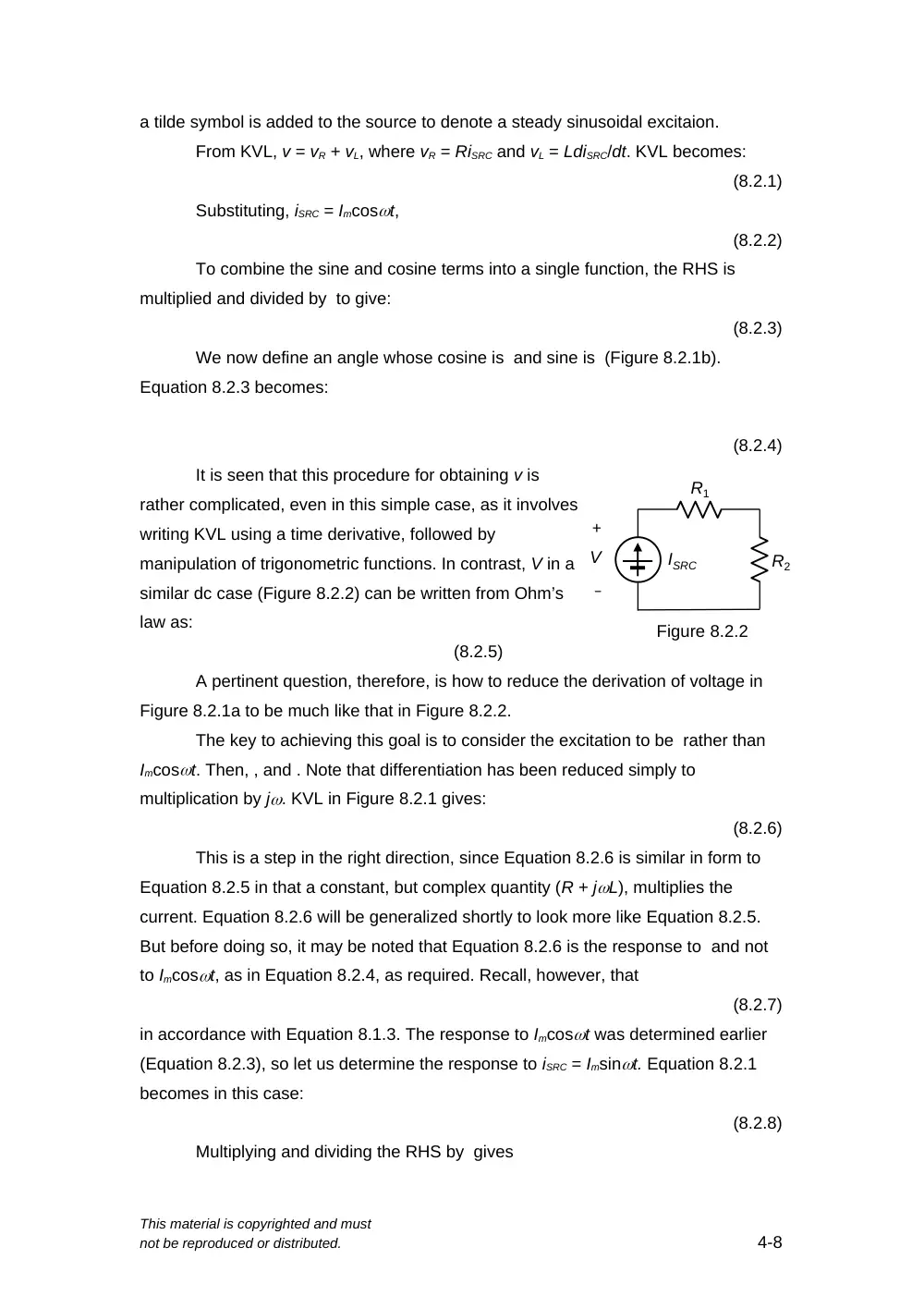Equation 8.2.3 becomes: (8.2.4) It is seen that this procedure for obtaining v is rather complicated, even in this simple case, as it involves writing KVL using a time derivative, followed by manipulation of trigonometric functions. In contrast, V in a similar dc case (Figure 8.2.2) can be written from Ohm’s law as: (8.2.5) A pertinent question, therefore, is how to reduce the derivation of voltage in Figure 8.2.1a to be much like that in Figure 8.2.2. The key to achieving this goal is to consider the excitation to be rather than Imcost. Then, , and . Note that differentiation has been reduced simply to multiplication by j. KVL in Figure 8.2.1 gives: (8.2.6) This is a step in the right direction, since Equation 8.2.6 is similar in form to Equation 8.2.5 in that a constant, but complex quantity (R + jL), multiplies the current. Equation 8.2.6 will be generalized shortly to look more like Equation 8.2.5. But before doing so, it may be noted that Equation 8.2.6 is the response to and not to Imcost, as in Equation 8.2.4, as required. Recall, however, that (8.2.7) in accordance with Equation 8.1.3. The response to Imcost was determined earlier (Equation 8.2.3), so let us determine the response to iSRC = Imsint. Equation 8.2.1 becomes in this case: (8.2.8) Multiplying and dividing the RHS by gives This material is copyrighted and must not be reproduced or distributed. 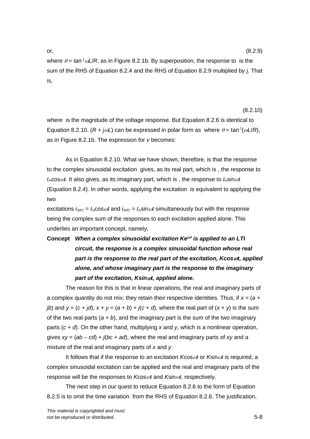4-8 or, (8.2.9) where  = tan-1L/R, as in Figure 8.2.1b. By superposition, the response to is the sum of the RHS of Equation 8.2.4 and the RHS of Equation 8.2.9 multiplied by j. That is, (8.2.10) where is the magnitude of the voltage response. But Equation 8.2.6 is identical to Equation 8.2.10. (R + jL) can be expressed in polar form as where  = tan-1(L/R), as in Figure 8.2.1b. The expression for v becomes: As in Equation 8.2.10. What we have shown, therefore, is that the response to the complex sinusoidal excitation gives, as its real part, which is , the response to Imcost. It also gives, as its imaginary part, which is , the response to Imsint (Equation 8.2.4). In other words, applying the excitation is equivalent to applying the two excitations iSRC = Imcost and iSRC = Imsint simultaneously but with the response being the complex sum of the responses to each excitation applied alone. This underlies an important concept, namely, Concept When a complex sinusoidal excitation Kejt is applied to an LTI circuit, the response is a complex sinusoidal function whose real part is the response to the real part of the excitation, Kcost, applied alone, and whose imaginary part is the response to the imaginary part of the excitation, Ksint, applied alone. The reason for this is that in linear operations, the real and imaginary parts of a complex quantity do not mix; they retain their respective identities. Thus, if x = (a + jb) and y = (c + jd), x + y = (a + b) + j(c + d), where the real part of (x + y) is the sum of the two real parts (a + b), and the imaginary part is the sum of the two imaginary parts (c + d). On the other hand, multiplying x and y, which is a nonlinear operation, gives xy = (ab – cd) + j(bc + ad), where the real and imaginary parts of xy and a mixture of the real and imaginary parts of x and y. It follows that if the response to an excitation Kcost or Ksint is required, a complex sinusoidal excitation can be applied and the real and imaginary parts of the response will be the responses to Kcost and Ksint, respectively. The next step in our quest to reduce Equation 8.2.6 to the form of Equation 8.2.5 is to omit the time variation from the RHS of Equation 8.2.6. The justification, This material is copyrighted and must not be reproduced or distributed. 5-8 Figure 8.2.3 (a)  Im Re Im (b)  Im Re  t ) (   j t me V t j me I  Im j t me V  V (c) R L  as explained earlier, is that when an LTI circuit is excited at a single frequency, all the currents and voltages in the circuit will be sinusoids having the same given frequency , but with different amplitudes and phase angles. No information is lost by omitting the time variation . This leads to phasor notation, as will be elaborated next. Phasor Notation The complex excitation and the complex response (Equation 8.2.10) can be plotted as position vectors on an Argand diagram (Figure 8.2.3a). Both vectors rotate counterclockwise at an angular speed , retaining the phase angle  between them as they do so. The angular speed is the same, because as emphasized earlier, all the voltage and current responses in an LTI circuit have the same frequency as the excitation. The information of interest in Figure 8.2.3a is the magnitude of the various vectors and their relative phase angle. It follows that no significant information is lost by freezing the rotation of the vectors at a particular value of t, which can be conveniently taken as t = 0. becomes , and becomes , as in Figure 8.2.3b. These complex quantities are referred to as phasors. Thus, Definition A phasor is a quantity such as Vmej representing a complex sinusoidal function of time, but with the time variation suppressed. Phasors are written in boldface and expressed as a magnitude and phase angle: V (8.2.11) It should be emphasized that phasors drawn in a given Argand diagram are implicitly complex sinusoidal functions of time rotating at the same angular frequency. Phasors that are implicitly rotating at different frequencies cannot, and should not, be dawn on the same Argand diagram. Nor should complex quantities, such as (R + jL) (Equation 8.2.6), be drawn on the same Argand diagram as phasors (Figure This material is copyrighted and must not be reproduced or distributed. 6-8 (c)   +  Y AY Y Im Im Re Re Y AY (a) Figure 8.2.5 Y   –  (b) Im Re A  Y/A 8.2.3c). Properties of Phasors Being geometrically position vectors, phasors have magnitude and direction, just like vectors, but with the additional property that their horizontal component is a real quantity, and their vertical component is an imaginary quantity. 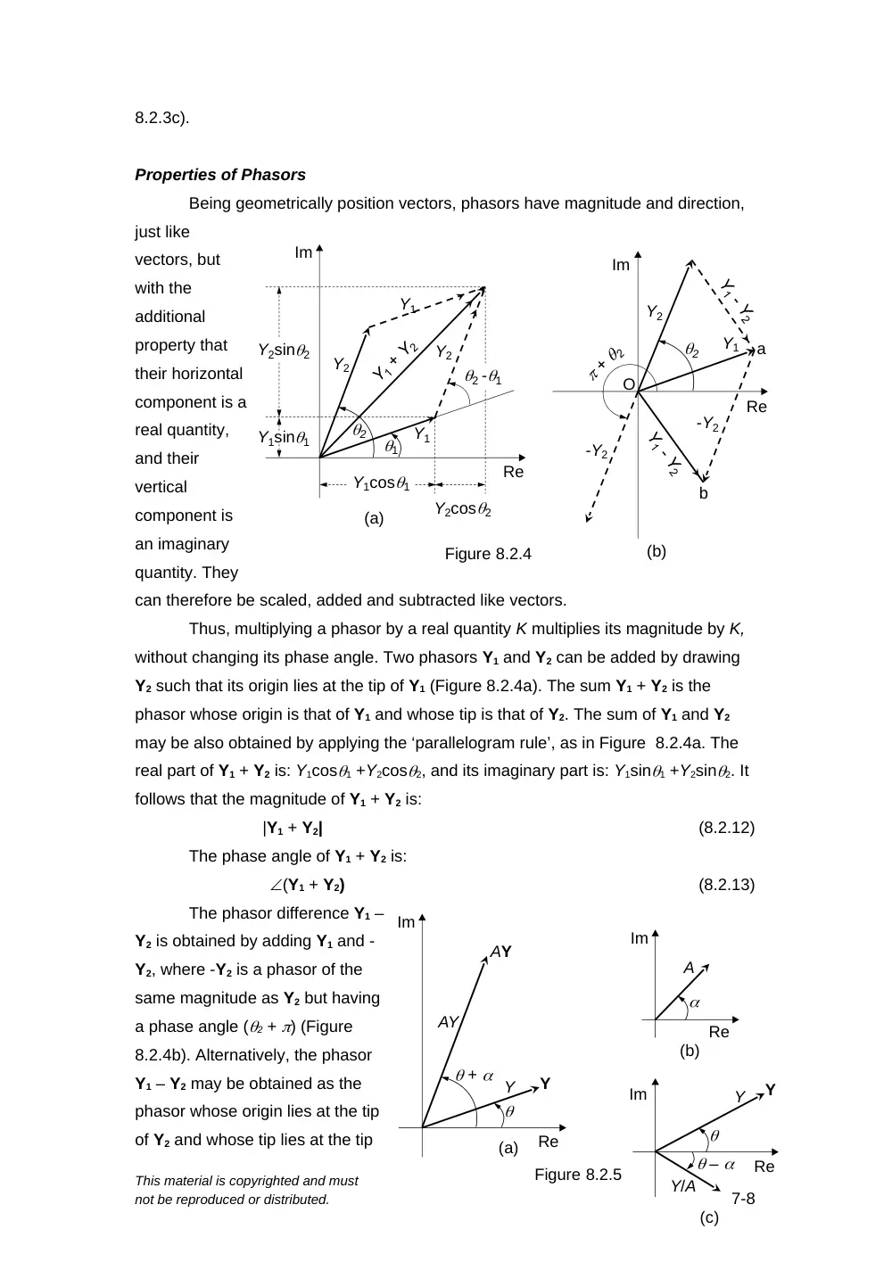They can therefore be scaled, added and subtracted like vectors. Thus, multiplying a phasor by a real quantity K multiplies its magnitude by K, without changing its phase angle. Two phasors Y1 and Y2 can be added by drawing Y2 such that its origin lies at the tip of Y1 (Figure 8.2.4a). The sum Y1 + Y2 is the phasor whose origin is that of Y1 and whose tip is that of Y2. The sum of Y1 and Y2 may be also obtained by applying the ‘parallelogram rule’, as in Figure 8.2.4a. The real part of Y1 + Y2 is: Y1cos1 +Y2cos2, and its imaginary part is: Y1sin1 +Y2sin2. It follows that the magnitude of Y1 + Y2 is: |Y1 + Y2| (8.2.12) The phase angle of Y1 + Y2 is: (Y1 + Y2) (8.2.13) The phasor difference Y1 – Y2 is obtained by adding Y1 and - Y2, where -Y2 is a phasor of the same magnitude as Y2 but having a phase angle (2 + ) (Figure 8.2.4b). Alternatively, the phasor Y1 – Y2 may be obtained as the phasor whose origin lies at the tip of Y2 and whose tip lies at the tip This material is copyrighted and must not be reproduced or distributed. 7-8 Figure 8.2.4 (a) (b) 1 2 2 -1 Y1 Y1 Y2 Y2 Y1cos1 Y2cos2 Y2sin2 Y1sin1 Y2 -Y2 Y1 -Y2 O a b Im Re Im Re 2 of Y1. Then: Y1 = Y2 + (Y1 – Y2). A phasor Y (Figure 8.2.5a) may be multiplied by a complex quantity (Figure 8.2.5b): (8.2.14) The product is a phasor of magnitude AY and phase angle ( +) (Figure 8.25a). A phasor Y may be divided by a complex quantity : (8.2.15) The quotient is a phasor of magnitude and phase angle ( –) (Figure 8.2.5c). 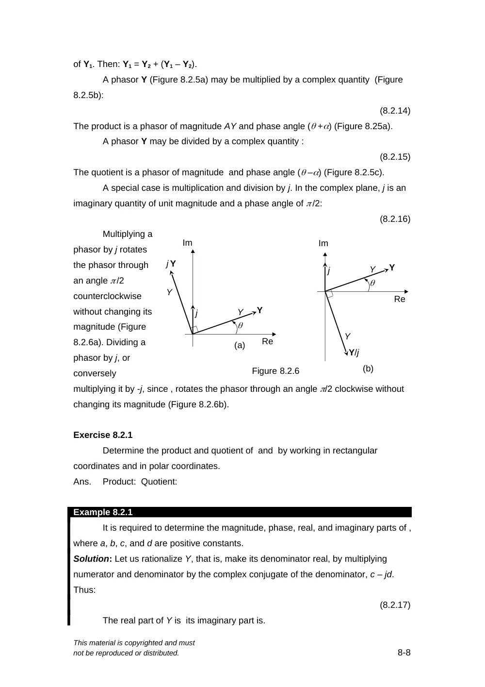A special case is multiplication and division by j. In the complex plane, j is an imaginary quantity of unit magnitude and a phase angle of  /2: (8.2.16) Multiplying a phasor by j rotates the phasor through an angle  /2 counterclockwise without changing its magnitude (Figure 8.2.6a). Dividing a phasor by j, or conversely multiplying it by -j, since , rotates the phasor through an angle /2 clockwise without changing its magnitude (Figure 8.2.6b). Exercise 8.2.1 Determine the product and quotient of and by working in rectangular coordinates and in polar coordinates. Ans. Product: Quotient: Example 8.2.1 It is required to determine the magnitude, phase, real, and imaginary parts of , where a, b, c, and d are positive constants. Solution: Let us rationalize Y, that is, make its denominator real, by multiplying numerator and denominator by the complex conjugate of the denominator, c – jd. Thus: (8.2.17) The real part of Y is its imaginary part is. This material is copyrighted and must not be reproduced or distributed. 8-8  Y Im Re Y (a) Figure 8.2.6 Y j Y j  Y Im Re Y (b) j Y Y/j The magnitude of Y may be obtained as the square root of the sum of the squares of the real and imaginary parts. An easier way is to convert the numerator and denominator to polar coordinates. Thus: . The magnitude of Y is therefore . The phase angle of Y is (1 – 2) = tan-1(b/a) – tan-1(d/c), that is, the phase angle is of the phase angle numerator minus that of the denominator. The following should be noted: i) Whereas the magnitude of Y is the magnitude of the numerator divided by that of the denominator, the real part of Y is not the real part of the numerator divided by that of the denominator. Nor is the imaginary part of Y the imaginary part of the numerator divided by that of the denominator. 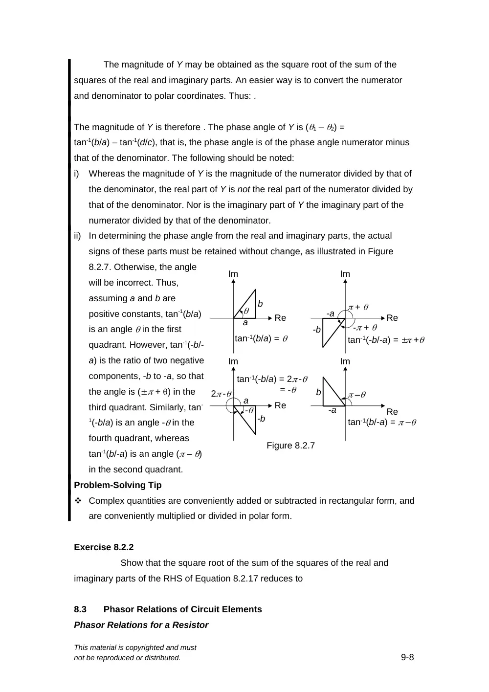ii) In determining the phase angle from the real and imaginary parts, the actual signs of these parts must be retained without change, as illustrated in Figure 8.2.7. Otherwise, the angle will be incorrect. Thus, assuming a and b are positive constants, tan-1(b/a) is an angle  in the first quadrant. However, tan-1(-b/- a) is the ratio of two negative components, -b to -a, so that the angle is ( + ) in the third quadrant. Similarly, tan- 1(-b/a) is an angle - in the fourth quadrant, whereas tan-1(b/-a) is an angle ( – ) in the second quadrant. Problem-Solving Tip  Complex quantities are conveniently added or subtracted in rectangular form, and are conveniently multiplied or divided in polar form. Exercise 8.2.2 Show that the square root of the sum of the squares of the real and imaginary parts of the RHS of Equation 8.2.17 reduces to 8.3 Phasor Relations of Circuit Elements Phasor Relations for a Resistor This material is copyrighted and must not be reproduced or distributed. 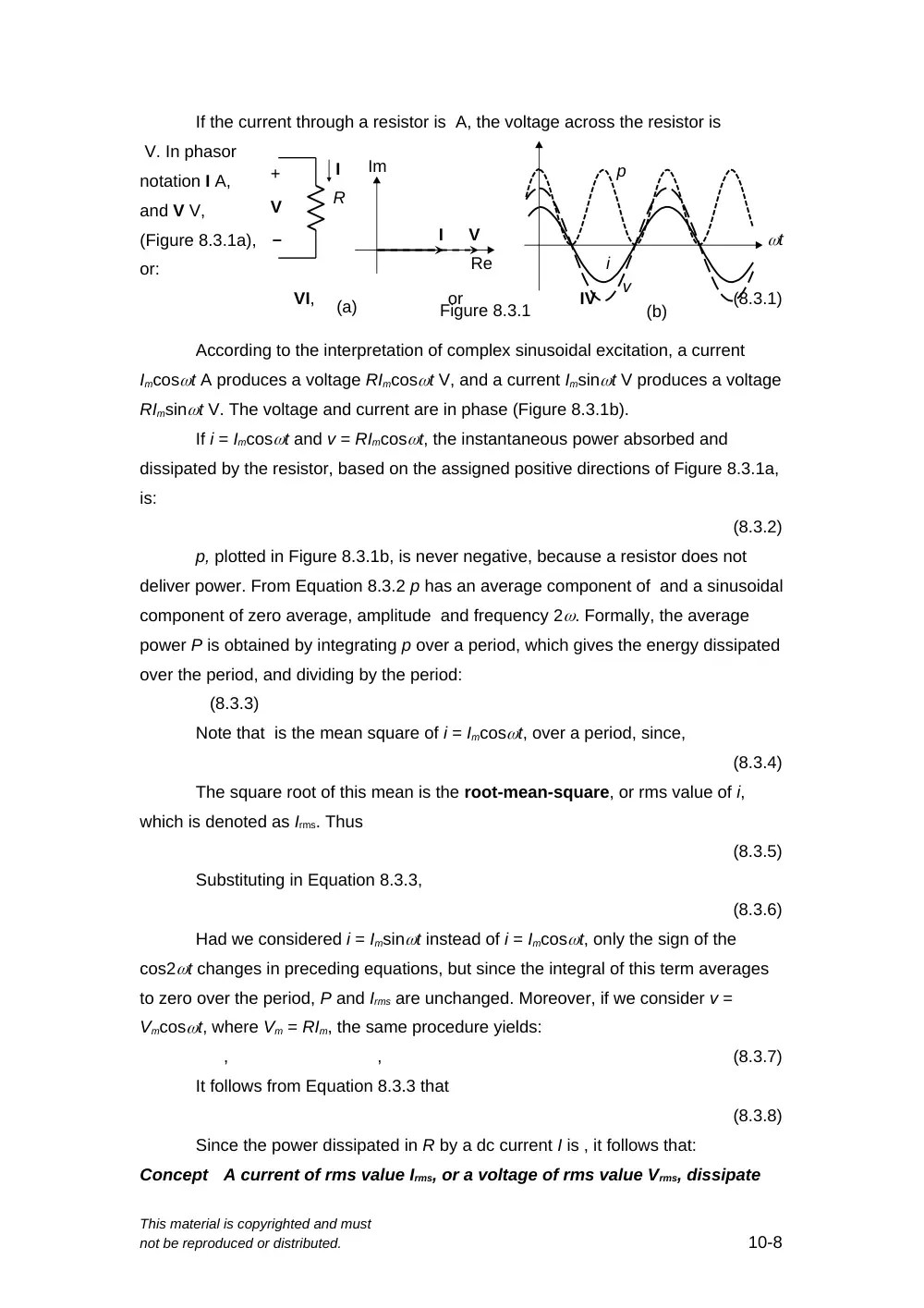9-8 a b  Im Re -a -b Im Re  +  tan-1(b/a) =  a -b - Im Re -a b Im Re  – tan-1(b/-a) =  – Figure 8.2.7 tan-1(-b/-a) =  + tan-1(-b/a) = 2 - = - 2 - - +  If the current through a resistor is A, the voltage across the resistor is V. In phasor notation I A, and V V, (Figure 8.3.1a), or: VI, or IV (8.3.1) According to the interpretation of complex sinusoidal excitation, a current Imcost A produces a voltage RImcost V, and a current Imsint V produces a voltage RImsint V. The voltage and current are in phase (Figure 8.3.1b). If i = Imcost and v = RImcost, the instantaneous power absorbed and dissipated by the resistor, based on the assigned positive directions of Figure 8.3.1a, is: (8.3.2) p, plotted in Figure 8.3.1b, is never negative, because a resistor does not deliver power. From Equation 8.3.2 p has an average component of and a sinusoidal component of zero average, amplitude and frequency 2. Formally, the average power P is obtained by integrating p over a period, which gives the energy dissipated over the period, and dividing by the period: (8.3.3) Note that is the mean square of i = Imcost, over a period, since, (8.3.4) The square root of this mean is the root-mean-square, or rms value of i, which is denoted as Irms. Thus (8.3.5) Substituting in Equation 8.3.3, (8.3.6) Had we considered i = Imsint instead of i = Imcost, only the sign of the cos2t changes in preceding equations, but since the integral of this term averages to zero over the period, P and Irms are unchanged. Moreover, if we consider v = Vmcost, where Vm = RIm, the same procedure yields: , , (8.3.7) It follows from Equation 8.3.3 that (8.3.8) Since the power dissipated in R by a dc current I is , it follows that: Concept A current of rms value Irms, or a voltage of rms value Vrms, dissipate This material is copyrighted and must not be reproduced or distributed. 10-8 V + R I (a) Figure 8.3.1 V I – Im Re (b) p v i t the same power in a given resistor as a dc current, or a dc voltage, of the same value. Using rms values of sinusoidal currents and voltages for power calculations results in expressions of the same form as under dc conditions. The rms value is also known as the effective value. Phasor Relations for a Capacitor If the current through a capacitor is A, the voltage across the capacitor is: (8.3.9) where K is the constant of integration that shifts the voltage in the vertical direction and defines its average value. When a sinusoidal current of zero average is applied to an uncharged capacitor, the resulting steady-state voltage is sinusoidal and of zero average, so that K = 0. In phasor notation, I A, and V V, or: VI or IV (8.3.10) (Figure 8.3.2a). The magnitude of V is (1/C) times that of I, and the phase angle of V is -90 (Figure 8.3.2a). According to the interpretation of complex sinusoidal excitation, a current Imcost A in a capacitor produces a voltage (Im/C)cos(t – /2) = (Im/C)sint across the capacitor, and a current Imsint A produces a voltage (Im/C)sin(t – /2) = (Im/C)cost. The voltage lags the current by 90, or the current leads the voltage by 90 (Figure 8.3.2). This can be ascertained by comparing the time of occurrence of the positive peaks of the waveforms of v and i in Figure 8.3.2b. Since the peak of v occurs later in time than the peak of i by a quarter of a period, v lags i by 90. The instantaneous power p absorbed by the capacitor is: (8.3.11) and, (8.3.12) p is plotted in Figure 8.3.2b. P = 0, because an ideal capacitor does not dissipate power. The power absorbed (p > 0) and stored as electric energy during a period is equal and opposite to the power delivered (p < 0), when the stored energy is returned to the supply over the period. This material is copyrighted and must not be reproduced or distributed. 11-8 (a) I V C j 1 I V + – Figure 8.3.2 Im Re (b) p v i t Phasor Relations for an Inductor If the inductor current is A, the inductor voltage is: (8.3.13) In phasor notation, I A, and V V, or: VI, or IV (8.3.14) The magnitude of V is L times that of I, and the phase angle of V is 90 (Figure 8.3.3a). According to the interpretation of complex sinusoidal excitation, a current Imcost A in the inductor produces a voltage LImcos(t + 90) = -LImsint across the inductor, and a current Imsint A produces a voltage LImsin(t – 90) = -LImcost. The voltage leads the current by 90, or the current lags the voltage by 90 (Figure 8.3.2(b)). This may be ascertained by comparing the time of occurrence of the positive peaks of the waveforms of v and i. Since the peak of v occurs earlier in time than the peak of i by a quarter of a period, v leads i by 90. The instantaneous power p absorbed by the inductor is: (8.3.15) and, (8.3.16) p, plotted in Figure 8.3.3b. P = 0, because an ideal inductor does not dissipate power. The power absorbed (p > 0) and stored as magnetic energy during a period is equal and opposite to the power delivered (p < 0), when the stored energy is returned to the supply over the period. From the preceding discussion, the v-i relations of capacitors and inductors in the time domain and in phasor notation are as follows: For a capacitor , and (8.3.17) For an inductor , and (8.3.18) It is seen that: Concept In phasor notation, differentiation in time is expressed as multiplication by j, and integration in time is expressed as division by j. Thus, differential and integral relations are transformed to algebraic relations in j for steady-state sinusoidal analysis ONLY. This concept in fact underlies the usefulness of phasor notation for steady- state sinusoidal analysis. This material is copyrighted and must not be reproduced or distributed. 12-8 jL (a) I V V + I – Figure 8.3.3 Im Re (b) p v i t Another important observation is that v and i are in phase for an ideal resistor but are in phase quadrature for ideal capacitors and inductors. This is because an ideal resistor only dissipates power. It does not store energy that must be returned later to the supply. If no power is delivered by an ideal resistor, p is never negative, which means that v and i are in phase. On the other hand, ideal capacitors and inductors do not dissipate power, which means that the average power P over a period is zero. For this to be the case, v and i must be in phase quadrature, which means that one is a cosine function and the other is a sine function, so that their product averages to zero over a period. Concept The sinusoidal voltage and current for an ideal resistor are in phase because such a resistor is purely dissipative. They are in phase quadrature for ideal energy storage elements because these elements are nondissipative. Exercise 8.3.1 The voltage applied to a resistor is peak, the frequency being 50 Hz. Determine: (a) the expression for the current in the time domain, assuming the voltage is a cosine function; and (b) the power dissipated in the resistor. Ans. (a) ; (b) 320 W. Exercise 8.3.2 The current through a series combination of a 10 mH inductor and a capacitor is rms. Assuming the frequency is 200 Hz and the time variation is a sine function, determine the expression in the time domain of the voltage across: (a) inductor; and (b) the capacitor. Ans. (a) 60sin(400t + 15) mV rms; (b) (750/) sin(400t –165) mV rms 8.4 Impedance and Reactance Let V = be a voltage phasor and I = be a related current phasor, representing, for example, the voltage and current between any two nodes in a circuit (Figure 8.4.1), and let . Then: Definition Impedance Z is the ratio of the voltage phasor Vm v between any two nodes in a circuit to the current phasor Im I flowing between these nodes in the direction of a voltage drop. This material is copyrighted and must not be reproduced or distributed. 13-8 Figure 8.4.1 V + I – = Z (8.4.1) (Figure 8.4.2a). When V is in volts and I is in amperes Z is in ohms. Since Z is in general complex, it can be expressed as: Z = R + jX (8.4.2) (Figure 8.4.2b). It should be emphasized that although Z is in general complex, it is not a phasor, because it is not a complex sinusoidal function of time in which the time variation has been suppressed. In fact, the exponential time variation cancels out in Equation 8.4.1. In the case of an ideal resistor, V and I are in phase (Equation 8.3.1), which means that Z is real and equal to R. It follows that R in Equation 8.4.2 is the usual resistance that we have considered in previous chapters, and that for an ideal resistor, X = 0. X, the imaginary part of Z, is the reactance and its unit is the ohm, just like resistance and impedance. For an ideal capacitor, Z = so that X = . For an ideal inductor, Equation 8.3.9 gives , so that . For both ideal energy storage elements, R = 0, since these elements are nondissipative. It should be emphasized that when X = 0, V and I are in phase. When X  0, Z is complex and V and I are out of phase. Hence: Concept In a purely resistive circuit, all sinusoidal voltages and currents are in phase and their magnitudes do not depend on frequency. Energy- storage storage elements possess reactance, which causes frequency-dependent phase differences between sinusoidal voltages and currents in the circuit and, in addition, makes the amplitudes of these sinusoidal voltages and currents depend on frequency. The following should be noted concerning reactance: 1. In any expression that involves impedance, reactance is always multiplied by j. For an ideal capacitor, X = -1/C and Z = -j/C. For an ideal inductor, X = L and Z = jL. 2. Since j appears in the V-I relations as a result of differentiating or integrating expressions involving e jt, j is always associated with  in the expression for impedance. Hence, reactance is always a function of frequency. The reciprocal of impedance is the admittance Y: (8.4.3) This material is copyrighted and must not be reproduced or distributed. 14-8 V R X (a) (b) Figure 8.4.2  Im Vm  I i v jB G Y Z    1  where B is the susceptance. Like G, B and Y are in siemens. For an ideal resistor, I/V = G (Equation 8.3.1), so that B = 0, and G is the usual conductance. For an ideal capacitor, Y = I/V = jC (Equation 8.3.7), so that G = 0 and B = jC. For an ideal inductor, Y = I/V = 1/jL =`-1/ (Equation 8.3.9), so that G = 0, and B = -1/L. Table 8.4.1 lists the circuit properties of the three circuit elements. It is seen that under dc conditions  = 0, which makes the reactance of a capacitor infinite and its susceptance zero. This means that when the voltage across the capacitor is dc, the current is zero. The capacitor behaves as an open circuit, as argued in Section 7.1, Chapter 7. Similarly, when  = 0, the reactance of an inductor is zero and its susceptance is infinite. This means that when the inductor current is dc, the voltage across the inductor is zero. The inductor behaves as a short circuit, as argued in Section 7.2, Chapter 7. Note that whereas G = 1/R for an ideal resistor, B = -1/X for an ideal capacitor or inductor. This is because conversion from reactance to susceptance must proceed through impedance and admittance, which introduces a minus sign in the reciprocal of the imaginary component. Thus, Z = jX, Y = 1/Z = 1/jX = -j/X. But Y = jB, so that B = -1/X. Exercise 8.4.1 Find the reactance and susceptance of (a) the inductor and (b) the capacitor of Exercise 8.3.2. Ans. (a) Inductor: , S; (b) Capacitor: -50/ ,  /50 S. Example 8.4.1 Given an impedance Zs = Rs + jLs, represented as Rs in series with Ls. It is required to determine Rp and Lp of the equivalent parallel combination (Figure 8.4.3). Solution: Since the two circuits are This material is copyrighted and must not be reproduced or distributed. 15-8 Rs Ls Rp Lp (a) (b) Figure 8.4.3 Zs Zp a b a b Table 8.4.1 Circuit Properties of Circuit Elements Circuit Property Resistor Inductor Capacitor Reactance (X) 0 L C   1 Impedance (Z) R jL C j j C    1  Susceptance (B) 0 L   1 C Admittance (Y) G = R 1 L j j L    1  jC equivalent between terminals ‘ab’, they must have the same V and I at these terminals, so that the ratio V/I is the same. This means that Zs = Zp = 1/Yp. It follows that: . Rationalizing this fraction by multiplying the numerator and denominator by the complex conjugate of the denominator, so as to make the denominator real, (8.4.4) Equating real and imaginary parts, and (8.4.5) From Table 8.4.1, Gp = 1/Rp and Bp = -1/Lp. It follows that: (8.4.6)