EECE 210 Chapter 3, Fall 2012

Chapter 3 Basic Analysis of Resistive Circuits 3.1 Number of Independent Circuit Equations  The circuit shown has 4 essential nodes, 7 essential branches, and 4 meshes. There are 14 circuit variables, that is, a current and a voltage for each essential branch. Hence, 14 simultaneous equations have to be written to solve for the unknown variables.  Seven equations are provided by the v-i relations for the branches. The number of equations provided by KCL and KVL is governed by the following relation between the number of essential branches B, the number of essential nodes N, and the number of meshes or independent loops L: B = L + (N – 1) (3.1.1)  (N – 1) in this equation is the number of independent essential nodes. In Figure 3.1.1, KCL applied to the (N – 1) independent essential nodes gives 3 equations whereas KVL applied to the L independent loops, or meshes, gives another 4 equations, thus providing the additional 7 independent equation required to solve for all the variables. 3.2 Node-Voltage Analysis Concept In node-voltage analysis, the unknown node voltages are assigned in such a manner that KVL is automatically satisfied. Equations based on KCL are then written for each independent node directly in terms of Ohm’s law.  Consider the bridge circuit of Figure 3.2.1, excited by a current source, with the resistors represented by conductances. One of the essential nodes, such as d, is arbitrarily chosen as the reference node, and the voltages of the other nodes are expressed with respect to this node. Thus, Va, Vb, and Vc are, respectively, the voltage drops from nodes a, b, and c to d. 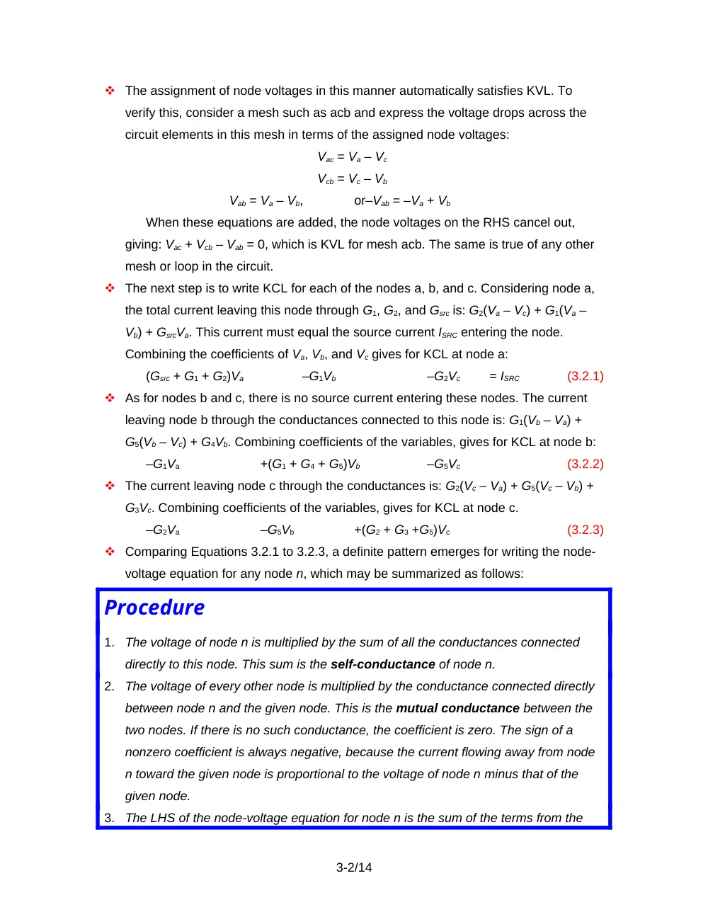3-1/14 VSRC a b c d R1 R2 R3 R4 R5 R6 R7 R8 Figure 3.1.1 +_ a a Va Vac Vab + + – –  The assignment of node voltages in this manner automatically satisfies KVL. To verify this, consider a mesh such as acb and express the voltage drops across the circuit elements in this mesh in terms of the assigned node voltages: Vac = Va – Vc Vcb = Vc – Vb Vab = Va – Vb, or–Vab = –Va + Vb When these equations are added, the node voltages on the RHS cancel out, giving: Vac + Vcb – Vab = 0, which is KVL for mesh acb. The same is true of any other mesh or loop in the circuit.  The next step is to write KCL for each of the nodes a, b, and c. Considering node a, the total current leaving this node through G1, G2, and Gsrc is: G2(Va – Vc) + G1(Va – Vb) + GsrcVa. This current must equal the source current ISRC entering the node. Combining the coefficients of Va, Vb, and Vc gives for KCL at node a: (Gsrc + G1 + G2)Va –G1Vb –G2Vc = ISRC (3.2.1)  As for nodes b and c, there is no source current entering these nodes. The current leaving node b through the conductances connected to this node is: G1(Vb – Va) + G5(Vb – Vc) + G4Vb. Combining coefficients of the variables, gives for KCL at node b: –G1Va +(G1 + G4 + G5)Vb –G5Vc (3.2.2)  The current leaving node c through the conductances is: G2(Vc – Va) + G5(Vc – Vb) + G3Vc. Combining coefficients of the variables, gives for KCL at node c. –G2Va –G5Vb +(G2 + G3 +G5)Vc (3.2.3)  Comparing Equations 3.2.1 to 3.2.3, a definite pattern emerges for writing the node- voltage equation for any node n, which may be summarized as follows: Procedure 1. The voltage of node n is multiplied by the sum of all the conductances connected directly to this node. This sum is the self-conductance of node n. 2. The voltage of every other node is multiplied by the conductance connected directly between node n and the given node. This is the mutual conductance between the two nodes. If there is no such conductance, the coefficient is zero. The sign of a nonzero coefficient is always negative, because the current flowing away from node n toward the given node is proportional to the voltage of node n minus that of the given node. 3. The LHS of the node-voltage equation for node n is the sum of the terms from the 3-2/14 preceding steps, ordered as the unknown node voltages. This sum is the total current leaving node n through the conductances connected to this node. 4. The RHS of the equation is equal to any source current entering node n.  Ideal resistors are bilateral, that is, the resistance is the same for both directions of current. This means that the mutual conductance terms in the equations of any two given nodes are the same. For example, the current flowing from node b toward node c is G5(Vb – Vc) in Figure 3.2.1, whereas the current flowing from node c toward node b is G5(Vc – Vb). The coefficient of Vc in the node-voltage equation for node b, which is –G5 in Equation 3.7.2, is the same as the coefficient of Vb in the node- voltage equation for node c (Equation 3.7.3). When ordered in a matrix, or array, the conductance coefficients are symmetrical with respect to the diagonal, in the absence of dependent sources. This is a useful check on the node-voltage equations. 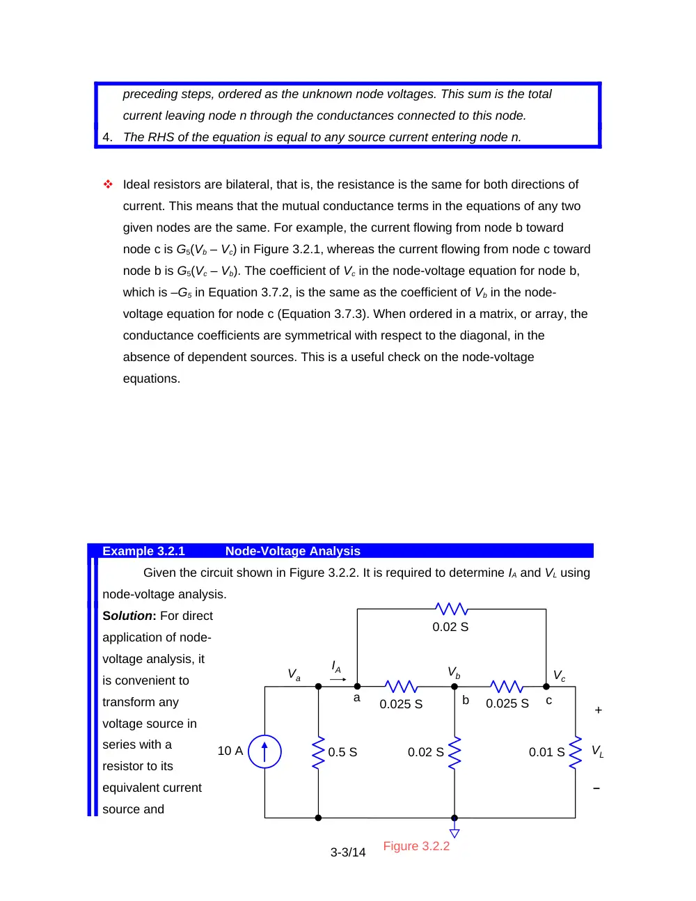Example 3.2.1 Node-Voltage Analysis Given the circuit shown in Figure 3.2.2. It is required to determine IA and VL using node-voltage analysis. Solution: For direct application of node- voltage analysis, it is convenient to transform any voltage source in series with a resistor to its equivalent current source and 3-3/14 0.01 S 10 A 0.025 S 0.02 S c Vc b Vb a IA 0.5 S 0.025 S 0.02 S Va Figure 3.2.2 VL + – represent resistors by their conductances. The lower node is chosen as the reference, since VL is with respect to this node. Following the procedure outlined above, the node- voltage equations for nodes a, b, and c, may be written directly: Va Vb Vc Va Vb Vc Va Vb Vc The conductance coefficients are symmetrical with respect to the diagonal. Simultaneous equations may be conveniently solved using MATLAB (Appendix SD.1). The solution is: Va = 19.3 V; Vb = 11.2 V; and Vc = 12.1 V. IA may be determined as the sum of the currents that flow into the 0.02 S and 0.025 S resistors connected to node a. That is, IA = = 0.346 A. Alternatively, IA = 10 – 0.5Va = 0.346 A. It is seen that VL = Vc = 12.1 V. 3.3 Special Considerations in Node-Voltage Analysis Dependent Sources  Dependent current sources in node-voltage analysis are treated exactly like independent sources. 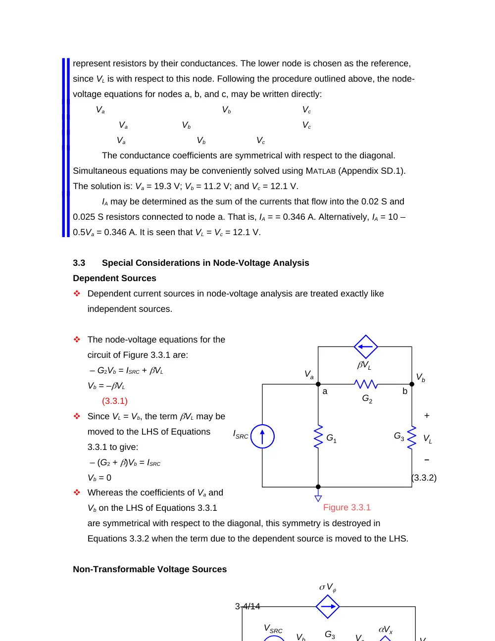 The node-voltage equations for the circuit of Figure 3.3.1 are: – G2Vb = ISRC + VL Vb = –VL (3.3.1)  Since VL = Vb, the term VL may be moved to the LHS of Equations 3.3.1 to give: – (G2 + )Vb = ISRC Vb = 0 (3.3.2)  Whereas the coefficients of Va and Vb on the LHS of Equations 3.3.1 are symmetrical with respect to the diagonal, this symmetry is destroyed in Equations 3.3.2 when the term due to the dependent source is moved to the LHS. Non-Transformable Voltage Sources 3-4/14 G2 G3 VL ISRC G1 a b Va Vb VL + Figure 3.3.1 – VSRC  V Vb Vx G3 Vc V  In the circuit of Figure 3.3.2, neither voltage source has a resistance directly in series with it, so it cannot be transformed to an equivalent current source.  However, if we choose node a as reference, Vb = VSRC, leaving three unknown node voltages: Vc, Vd, and Ve.  The node equation for node e is: (3.3.3)  Since the current through the dependent voltage source  Vx is not known. An unknown current I is introduced, which is arbitrarily assigned a direction from node c to node d. The equation for node c is: = – I (3.3.4)  The equation for node d is: = I +  V (3.3.5)  I is eliminated by adding Equations 3.3.4 and 3.3.5 together: =  V (3.3.6)  The third equation is the voltage relation for the dependent voltage source:  Vx (3.3.7)  Substituting Vb = VSRC and , and rearranging the variables, gives three equations that may be solved for , , and : VSRC (3.3.8) VSRC (3.3.9)  VSRC (3.3.10) Change of Reference Node  If node e is grounded and voltages are required with respect to node e, then all we have to do is subtract the value of Ve from all the node voltages determined with node a as reference. If for the circuit of Figure 3.3.2, Va = 0, Vb = 20 V, Vc = 12.5 V, Vd = 18.5 V, and Ve = 7.97 V, then if node e is grounded, Va = -7.97 V, Vb = 12.0 V, Vc = 4.51 V, Vd =10.5 V, and Ve = 0.  The justification is simply that the branch voltages, which are the basic quantities uniquely associated with the branch currents, depend on the difference between the node voltages at the ends of a given branch and are not changed by adding the same constant voltage to all the node voltages. 3-5/14 3.4 Mesh-Current Analysis Concept In mesh-current analysis, the unknown mesh currents are assigned in such a manner that KCL is automatically satisfied. Equations based on KVL are then written for each mesh directly in terms of Ohm’s law. 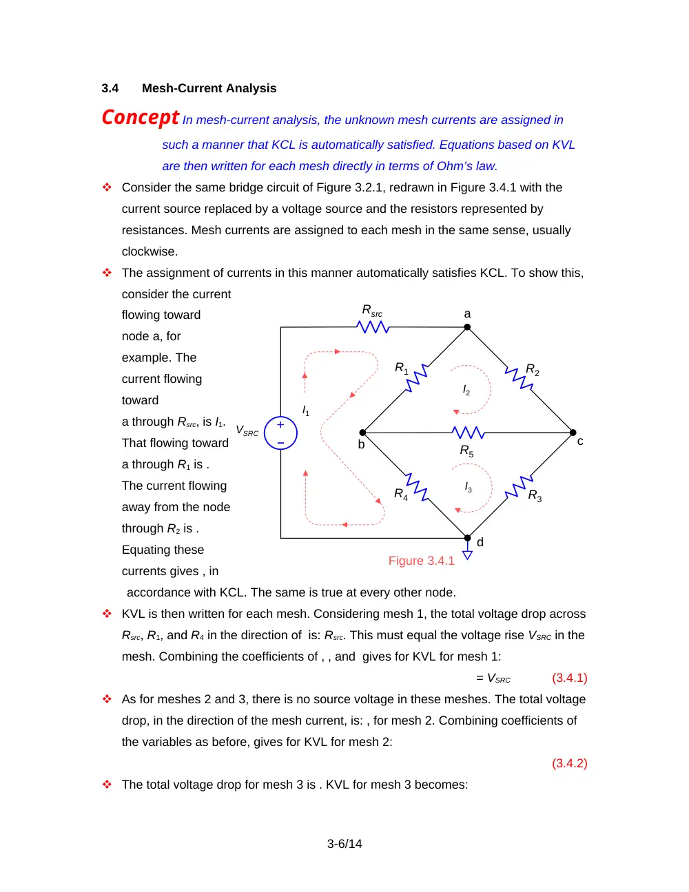 Consider the same bridge circuit of Figure 3.2.1, redrawn in Figure 3.4.1 with the current source replaced by a voltage source and the resistors represented by resistances. Mesh currents are assigned to each mesh in the same sense, usually clockwise.  The assignment of currents in this manner automatically satisfies KCL. To show this, consider the current flowing toward node a, for example. The current flowing toward a through Rsrc, is I1. That flowing toward a through R1 is . The current flowing away from the node through R2 is . Equating these currents gives , in accordance with KCL. The same is true at every other node.  KVL is then written for each mesh. Considering mesh 1, the total voltage drop across Rsrc, R1, and R4 in the direction of is: Rsrc. This must equal the voltage rise VSRC in the mesh. Combining the coefficients of , , and gives for KVL for mesh 1: = VSRC (3.4.1)  As for meshes 2 and 3, there is no source voltage in these meshes. The total voltage drop, in the direction of the mesh current, is: , for mesh 2. Combining coefficients of the variables as before, gives for KVL for mesh 2: (3.4.2)  The total voltage drop for mesh 3 is . 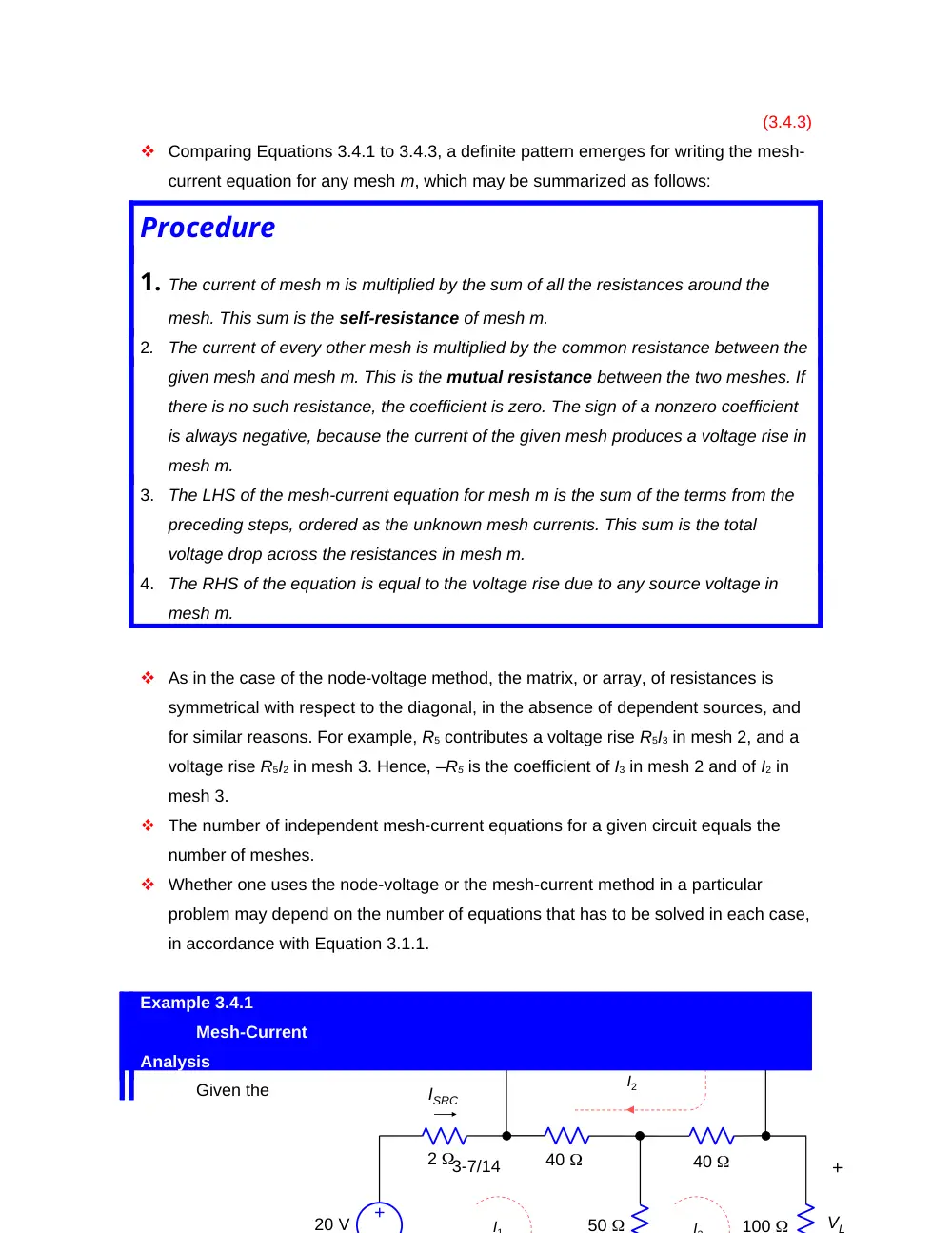KVL for mesh 3 becomes: 3-6/14 R5 R1 R2 R3 R4 Figure 3.4.1 a b c d VSRC – + Rsrc I1 I2 I3 ISRC 40  50  VL + 50  100  40  + 20 V I3 I1 I2 2  (3.4.3)  Comparing Equations 3.4.1 to 3.4.3, a definite pattern emerges for writing the mesh- current equation for any mesh m, which may be summarized as follows: Procedure 1. The current of mesh m is multiplied by the sum of all the resistances around the mesh. This sum is the self-resistance of mesh m. 2. The current of every other mesh is multiplied by the common resistance between the given mesh and mesh m. This is the mutual resistance between the two meshes. If there is no such resistance, the coefficient is zero. The sign of a nonzero coefficient is always negative, because the current of the given mesh produces a voltage rise in mesh m. 3. The LHS of the mesh-current equation for mesh m is the sum of the terms from the preceding steps, ordered as the unknown mesh currents. This sum is the total voltage drop across the resistances in mesh m. 4. The RHS of the equation is equal to the voltage rise due to any source voltage in mesh m.  As in the case of the node-voltage method, the matrix, or array, of resistances is symmetrical with respect to the diagonal, in the absence of dependent sources, and for similar reasons. For example, R5 contributes a voltage rise R5I3 in mesh 2, and a voltage rise R5I2 in mesh 3. Hence, –R5 is the coefficient of I3 in mesh 2 and of I2 in mesh 3.  The number of independent mesh-current equations for a given circuit equals the number of meshes.  Whether one uses the node-voltage or the mesh-current method in a particular problem may depend on the number of equations that has to be solved in each case, in accordance with Equation 3.1.1. Example 3.4.1 Mesh-Current Analysis Given the 3-7/14 same circuit of Figure 3.2.2. It is required to determine ISRC and VL using mesh-current analysis. Solution: The circuit is redrawn in Figure 3.4.2 showing the mesh currents. The 10 A source in combination with the 0.5 S is transformed to a voltage source of 20 V in series with 2 . Following the procedure outlined above, the mesh-current equations for meshes 1, 2, and 3 are: The resistance coefficients are symmetrical with respect to the diagonal. Solving these equations gives: A; A; A. Hence, I3V, and I1 = IA, as in Example 3.2.1. 3.5 Special Considerations in Mesh-Current Analysis Dependent Sources. 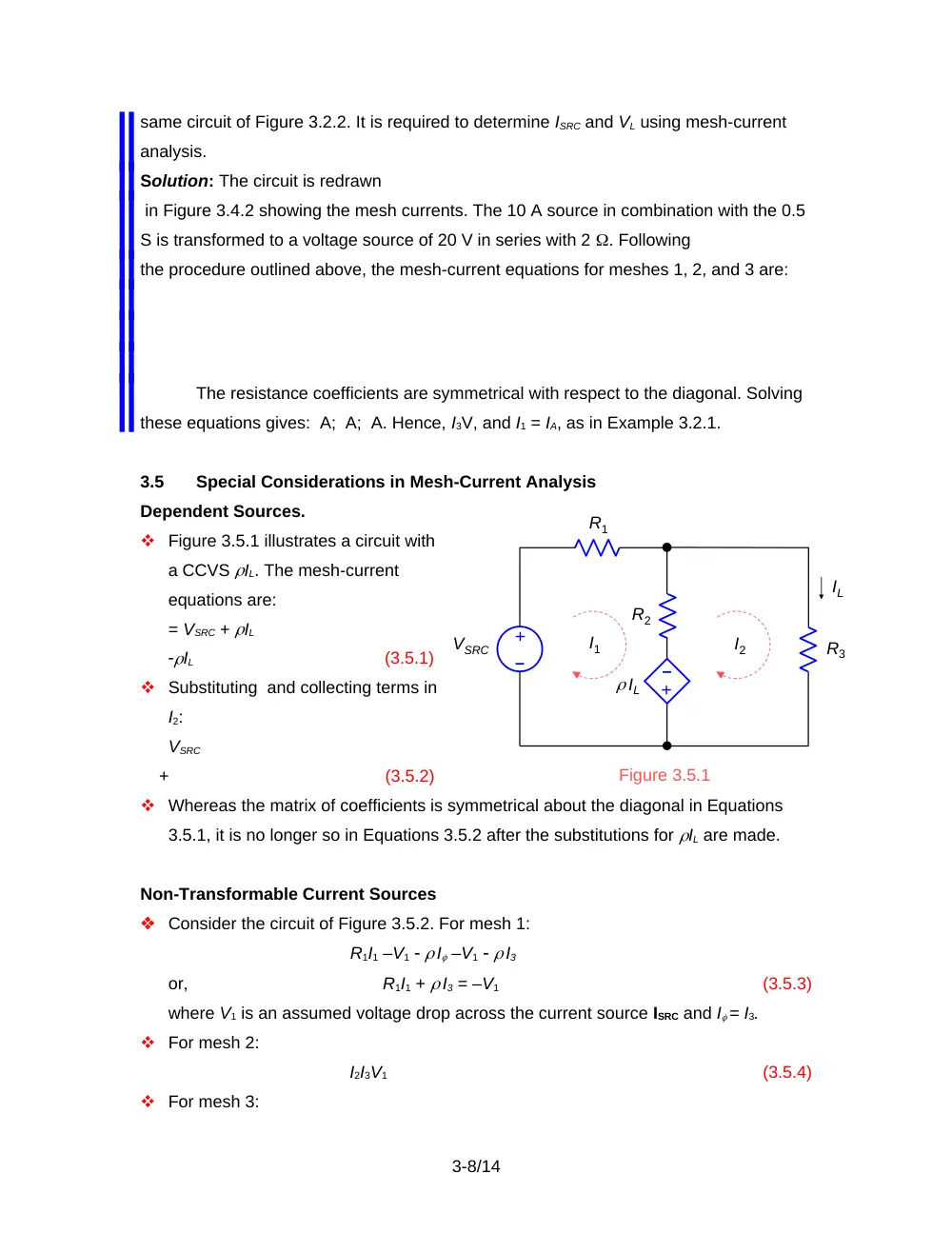 Figure 3.5.1 illustrates a circuit with a CCVS IL. The mesh-current equations are: = VSRC + IL IL (3.5.1)  Substituting and collecting terms in I2: VSRC + (3.5.2)  Whereas the matrix of coefficients is symmetrical about the diagonal in Equations 3.5.1, it is no longer so in Equations 3.5.2 after the substitutions for IL are made. 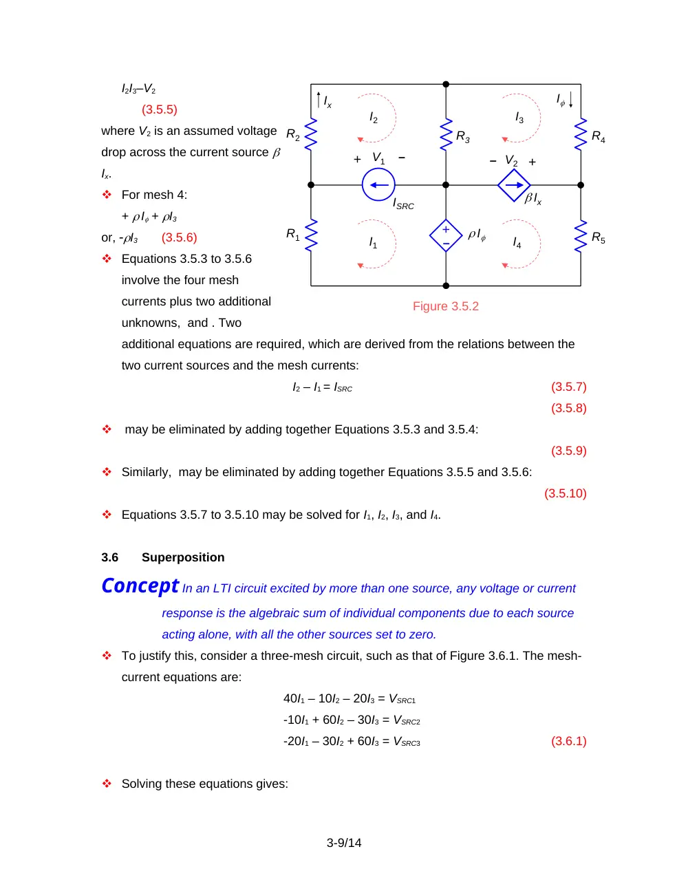Non-Transformable Current Sources  Consider the circuit of Figure 3.5.2. For mesh 1: R1I1 –V1   I –V1   I3 or, R1I1 +  I3 = –V1 (3.5.3) where V1 is an assumed voltage drop across the current source ISRC and I = I3.  For mesh 2: I2I3V1 (3.5.4)  For mesh 3: 3-8/14 R1 R2 R3 IL  IL VSRC – + – + I1 I2 Figure 3.5.1 I2I3–V2 (3.5.5) where V2 is an assumed voltage drop across the current source  Ix.  For mesh 4: +  I + I3 or, I3 (3.5.6)  Equations 3.5.3 to 3.5.6 involve the four mesh currents plus two additional unknowns, and . Two additional equations are required, which are derived from the relations between the two current sources and the mesh currents: I2 – I1 = ISRC (3.5.7) (3.5.8)  may be eliminated by adding together Equations 3.5.3 and 3.5.4: (3.5.9)  Similarly, may be eliminated by adding together Equations 3.5.5 and 3.5.6: (3.5.10)  Equations 3.5.7 to 3.5.10 may be solved for I1, I2, I3, and I4. 3.6 Superposition Concept In an LTI circuit excited by more than one source, any voltage or current response is the algebraic sum of individual components due to each source acting alone, with all the other sources set to zero. 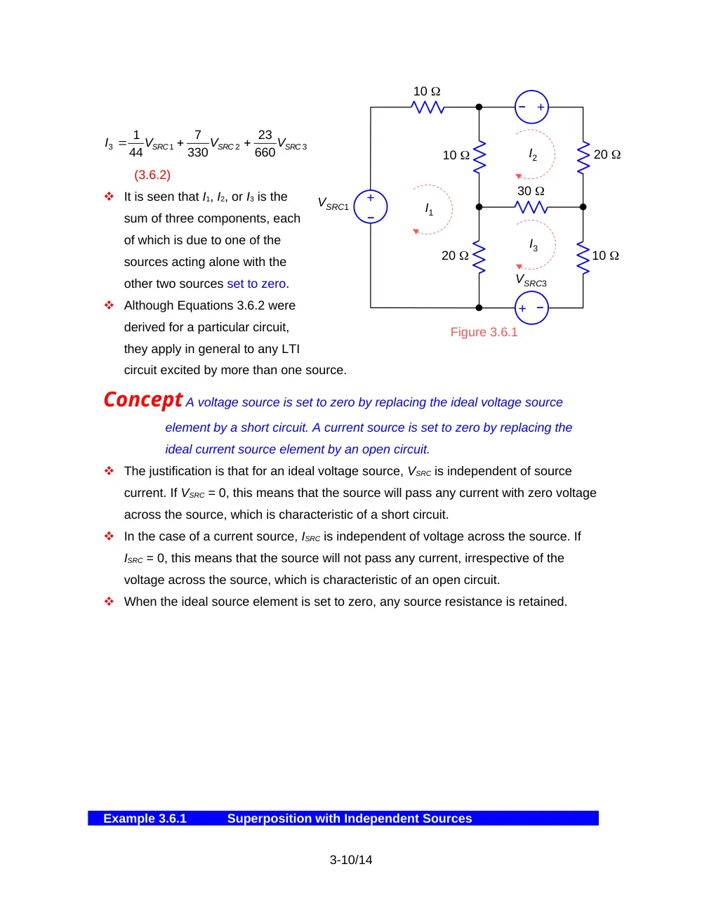 To justify this, consider a three-mesh circuit, such as that of Figure 3.6.1. The mesh- current equations are: 40I1 – 10I2 – 20I3 = VSRC1 -10I1 + 60I2 – 30I3 = VSRC2 -20I1 – 30I2 + 60I3 = VSRC3 (3.6.1)  Solving these equations gives: 3-9/14 Figure 3.5.2 + R5 R4 + R3 R2 R1 – – + – ISRC I2 I  I Ix I1 I3 I4  Ix V1 V2 10  VSRC1 – + I1 I2 Figure 3.6.1 – + – + I3 10  10  20  30  20  VSRC3 (3.6.2)  It is seen that I1, I2, or I3 is the sum of three components, each of which is due to one of the sources acting alone with the other two sources set to zero.  Although Equations 3.6.2 were derived for a particular circuit, they apply in general to any LTI circuit excited by more than one source. Concept A voltage source is set to zero by replacing the ideal voltage source element by a short circuit. A current source is set to zero by replacing the ideal current source element by an open circuit.  The justification is that for an ideal voltage source, VSRC is independent of source current. If VSRC = 0, this means that the source will pass any current with zero voltage across the source, which is characteristic of a short circuit.  In the case of a current source, ISRC is independent of voltage across the source. If ISRC = 0, this means that the source will not pass any current, irrespective of the voltage across the source, which is characteristic of an open circuit.  When the ideal source element is set to zero, any source resistance is retained. Example 3.6.1 Superposition with Independent Sources 3-10/14 3 2 1 3 660 23 330 7 44 1 SRC SRC SRC V V V I    It is required to determine VO in the circuit of Figure 3.6.2 using superposition. Solution: If the current source is replaced by an open circuit, the resistance between terminals ab is 30|| 60 = 20 . Hence, V, and VO1 = 12 V, where VO1 is the component of VO due to the voltage source acting alone. If the voltage source is replaced by a short circuit, the resistance between terminals ab is 10||30 = 7.5 . The resistance in parallel with the 40  is 27.5 , and the resistance across the current source is (27.5)||40 = . Hence, VO2 = 44 V, where VO2 is the component of VO due to the current source acting alone. By superposition, VO = 12 + 44 = 56 V. Dependent Sources  In the presence of dependent sources, superposition can be applied in one of two ways, depending on which method is easier to apply:  If we consider that the VSRC’s on the RHS of Equations 3.6.1 are due to independent sources only, then the effect of dependent sources is to modify the resistance coefficients on the LHS. The implication is that when applying superposition, dependent sources should remain unaltered.  The dependent source may be replaced by an independent source of assigned, symbolic value. Superposition is applied and a relation derived for the desired circuit variable in terms of the assigned value. This relation can then be used with the dependence relation of the source to solve the problem. In some problems, this is the quicker solution. Example 3.6.2 Superposition with Dependent Sources Given the circuit of Figure 3.6.3. It is required to find VO using superposition. 3-11/14 10  27 V 40  20  + – VO + – 2.7 A 30  Figure 3.6.2 a b + 20  0.5IO A + – + 20 V Solution: (a) Leaving the dependent source unaltered. In this case, each of the two voltage sources is replaced by a short circuit, one at a time, and the two components of VO determined. If the 20 V source is replaced by a short circuit, the circuit becomes as shown in Figure 3.6.4a. Let VO1 be the component of VO and IO1 be the current in the leftmost 10  resistor, where VO1 = 10IO1. The current in the rightmost 10  resistor is also IO1, because the same voltage VO1 is across this resistor. The current flowing away from node b through the two 10  resistors is 2IO1. Since 0.5IO1 flows toward node b from the dependent source, it follows from KCL that a current 1.5IO1 flows toward node b through the 20  resistor. Applying KVL to the mesh abca: , or VO1 = 10 V. When the 40 V source is replaced by a short circuit, the circuit becomes as shown in Figure 3.6.4b. Let VO2 be the component of VO and IO2 be the current in the leftmost 10  resistor, where VO2 = 10IO2. Since VO2 is also across the 20  resistor, the current through this resistor is 0.5IO2. From KCL at node b, the current through the 20 V source is 1.5IO2. as shown. From KCL at node d, the current in the rightmost 10  resistor is IO2 directed upward. Hence, the voltage across this resistor is also VO2 in the polarity shown. Applying KVL to the mesh bcd gives 20 = 2VO2, or VO2 = 10 V. From superposition, VO = VO1 + VO2 = 20 V. (b) Dependent source treated as an independent source. The dependent source is assigned a value, say Ix as an independent source (Figure 3.6.5) and superposition is applied with each of the three sources acting alone. When the 3-12/14 – + 40 V 20  IO1 0.5IO1 A + – VO1 10  10  (a) IO1 0.5IO1 1.5IO1 a b c Figure 3.6.4 20  IO2 0.5IO2 A + – VO2 – + 10  10  20 V (b) 0.5IO2 b c 1.5IO2 IO2 0.5IO2 d + – VO2 + 20  Ix + V – + 20 V 40 V source is applied alone, with the 20 V replaced by a short circuit and Ix by an open circuit, 8 V. When the 20 V source is applied alone, with the 40 V replaced by a short circuit and Ix by an open circuit, V. When Ix is applied alone, with the two voltage sources replaced by short circuits, VO3 = (10||10||20)Ix. To calculate the parallel resistance, the two 10  resistors in parallel give 5 . This resistance in parallel with 20  is 4, so that VO3 = 4Ix. It follows that VO = VO1 + VO2 + VO3 = 16 + 4Ix. From the original circuit (Figure 3.6.3), , so that . Substituting, gives V, as before. Power with Superposition Concept In a circuit excited by more than one source, the total power dissipated in a given resistor is NOT the sum of the powers due to each source acting alone, with all the other sources set to zero.  The reason is that the power dissipated in a given resistor is proportional to the square of the current through the resistor, or the square of the voltage across it, and the sum of the squares of a set of quantities is not equal to the square of the sum of these quantities. Thus, in Example 3.6.2, part(a), VO1 = VO2 = 10 V. The sum of the powers due to these components is W. The true power dissipated is W. Scaling of Input Concept In a circuit excited by a single independent source, multiplying the excitation by a constant K, multiplies all the voltage and current responses by the same constant.  If only a single excitation, say , is applied to the circuit of Figure 3.6.1, Equations 3.6.2 become, with VSRC2 = VSRC3 = 0: , (3.6.3)  If VSRC1 is multiplied by K, then I1, I2, and I3 are also multiplied by K. This fact may be usefully exploited in some problems by working backwards. That is, rather than determine the output for a given input, a convenient output is assumed and the input that produces this output is determined. The desired output is then obtained by simple scaling according to the given input Example 3.6.3 Scaling Applied to a Ladder Circuit It is required to 3-13/14 20 V + – 1  1  1  1  1  1  IO determine IO in the ladder circuit of Figure 3.6.7. Solution: The quickest way to solve this problem is to assume a convenient value for IO and work backwards towards the source. If IO = 1 A (Figure 3.6.8), Vcc’ = 3 V and the current in the cc’ branch is 3 A. The current in the bc and c’b’ branches is 4 A, and Vbb’ = 11 V. That makes the source current 15 A, and the source voltage 41 V. But the given source is 20 V; so the actual value of IO is A. Excitation by Dependent Sources  It follows from Equations 3.6.2 that if the circuit has dependent sources only, then all the VSRC’s are zero and hence all the responses are zero.  In Figure 3.6.9, for example, , and . Substituting, , which is impossible unless V = 0. This means that the source current is zero and all responses in the circuit are zero.  In some cases, dependent sources can make the circuit unstable and the response theoretically increases with time without limit. Hence, a more accurate statement is: Concept In a stable LTI circuit containing dependent sources, and no independent sources, all circuit responses are zero. 3-14/14 Figure 3.6.9 3  – +  V V 3 3  3  a b 41 V 15 A 11A 1 A 4 A 3 A 15 A 4 A c c b b + – Figure 3.6.8