EECE 210 Chapter 4, Fall 2012

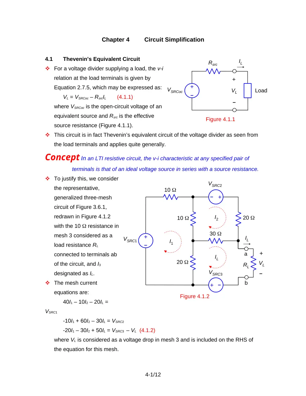
Chapter 4 Circuit Simplification 4.1 Thevenin’s Equivalent Circuit  For a voltage divider supplying a load, the v-i relation at the load terminals is given by Equation 2.7.5, which may be expressed as: VL = VSRCoc – RsrcIL (4.1.1) where VSRCoc is the open-circuit voltage of an equivalent source and Rsrc is the effective source resistance (Figure 4.1.1).  This circuit is in fact Thevenin’s equivalent circuit of the voltage divider as seen from the load terminals and applies quite generally. Concept In an LTI resistive circuit, the v-i characteristic at any specified pair of terminals is that of an ideal voltage source in series with a source resistance.  To justify this, we consider the representative, generalized three-mesh circuit of Figure 3.6.1, redrawn in Figure 4.1.2 with the 10  resistance in mesh 3 considered as a load resistance RL connected to terminals ab of the circuit, and I3 designated as IL.  The mesh current equations are: 40I1 – 10I2 – 20IL = VSRC1 -10I1 + 60I2 – 30IL = VSRC2 -20I1 – 30I2 + 50IL = VSRC3 – VL (4.1.2) where VL is considered as a voltage drop in mesh 3 and is included on the RHS of the equation for this mesh. 4-1/12 Figure 4.1.1 Rsrc – + + – VL Load VSRCoc IL 10  VSRC1 – + I1 I2 Figure 4.1.2 – + – + IL 10  RL 20  30  20  VSRC2 VSRC3 – + VL IL a b  Solving for IL and rearranging: (4.1.3)  Equation 4.1.3 is of the form of Eq 4.1.1, where VSRCoc equals the bracketed terms, and Rsrc = 430/23. Since the circuit of Figure 4.1.2 is quite arbitrary, it is concluded that the v-i relation for any given circuit at specified terminals ab is the same, in general, as that of an ideal voltage source VSRCoc in series with a resistance Rsrc.  The VSRCoc-Rsrc circuit is the TEC of the given circuit at terminals ab and is the simplest possible equivalent circuit, since it consists of just an ideal source and a resistor. It is customary to refer to VSRCoc as the Thevenin voltage VTh, and to Rsrc as the Thevenin resistance RTh.  VTh is determined as the open-circuit voltage at specified pair of terminals. If terminals ab in Figure 4.1.2 are open circuited, IL = 0 and the mesh current equations for the circuit become: 40I1 – 10I2 = VSRC1 -10I1 + 60I2 = VSRC2 (4.1.4)  Solving for I1 and I2, and . From KVL, VL = 30I2 + 20I1 + VSRC3. This gives: (4.1.5) which is the open-circuit voltage determined above. 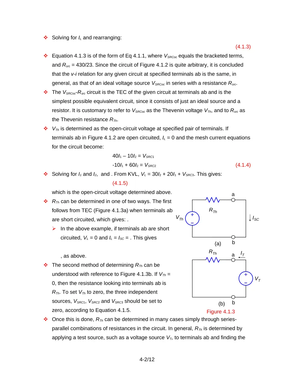 RTh can be determined in one of two ways. The first follows from TEC (Figure 4.1.3a) when terminals ab are short circuited, which gives: .  In the above example, if terminals ab are short circuited, VL = 0 and IL = ISC = . This gives , as above.  The second method of determining RTh can be understood with reference to Figure 4.1.3b. If VTh = 0, then the resistance looking into terminals ab is RTh. To set VTh to zero, the three independent sources, VSRC1, VSRC2 and VSRC3 should be set to zero, according to Equation 4.1.5.  Once this is done, RTh can be determined in many cases simply through series- parallel combinations of resistances in the circuit. In general, RTh is determined by applying a test source, such as a voltage source VT, to terminals ab and finding the 4-2/12 Figure 4.1.3 RTh – + VTh ISC a b RTh – + IT a b VT (a) (b) Figure 4.1.4 RN + – VL Load IN IL resulting current IT as a function of VT.  In summary: Procedure The derivation of TEC of a given circuit between a specified pair of terminals involves in general the following steps: 1. Determining the open-circuit voltage VTh at the specified terminals. 2. Determining the short-circuit current ISC at the specified terminals. 3. Setting independent sources to zero and determining the resistance RTh looking into the specified terminals. RTh is then determined either directly, or by applying a test voltage and finding the test current. Since VTh = RThISC, only two of the three quantities in this relation need be determined through the above steps. However, it is useful for checking purposes to determine all three independently.  Dependent sources affect the resistance values in the circuit. They should not be set to zero in determining RTh, as this will change the circuit. Norton’s Equivalent Circuit.  When the source VTh, in conjunction with RTh, is transformed to an equivalent current source, Norton’s equivalent circuit (NEC) is obtained (Figure 4.1.4). 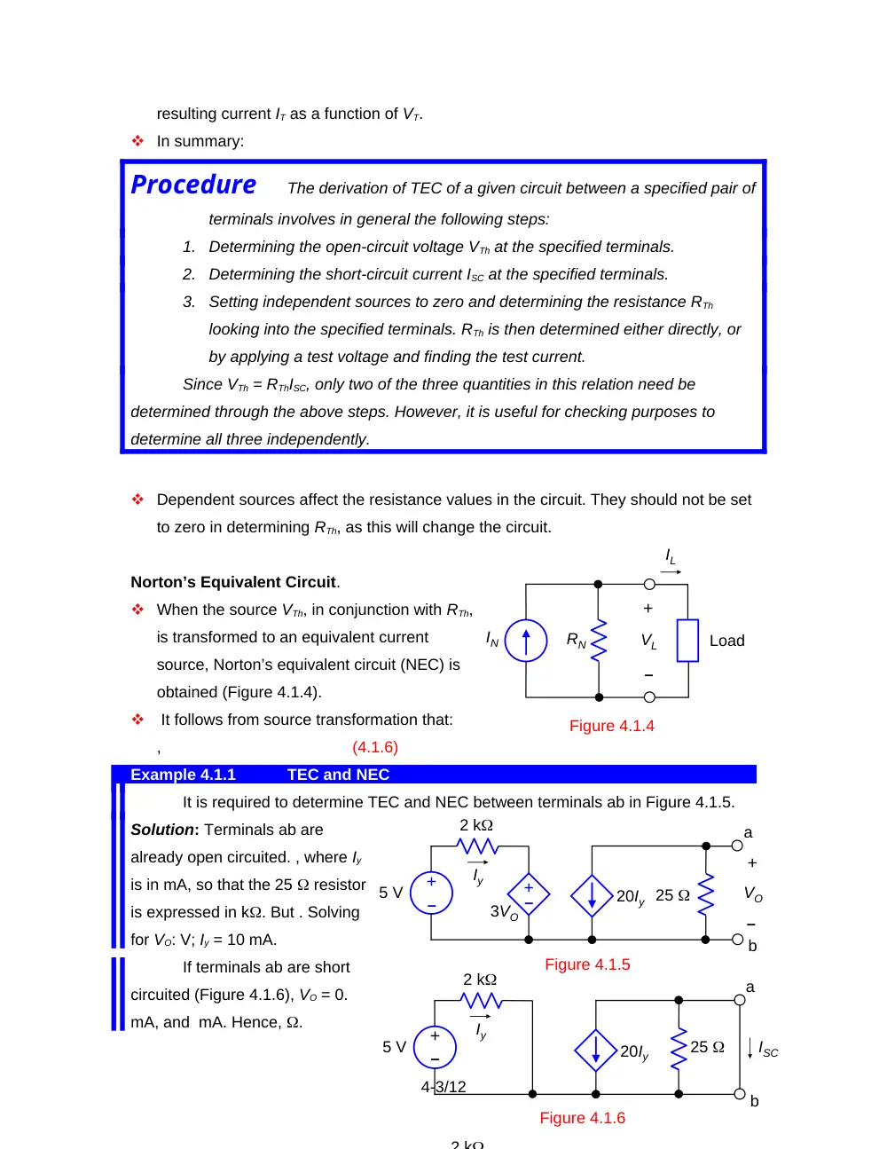 It follows from source transformation that: , (4.1.6) Example 4.1.1 TEC and NEC It is required to determine TEC and NEC between terminals ab in Figure 4.1.5. Solution: Terminals ab are already open circuited. , where Iy is in mA, so that the 25  resistor is expressed in k. But . Solving for VO: V; Iy = 10 mA. If terminals ab are short circuited (Figure 4.1.6), VO = 0. mA, and mA. Hence, . 4-3/12 – + 25  5 V 2 k Iy – + 3VO 20Iy + – VO a b Figure 4.1.5 – + 5 V 2 k Iy 20Iy a b ISC Figure 4.1.6 25  2 k If VT is applied, with the 5 V source replaced by a short circuit (Figure 4.1.7), Iy = . From KCL at node a, IT = . Hence, k  100 . 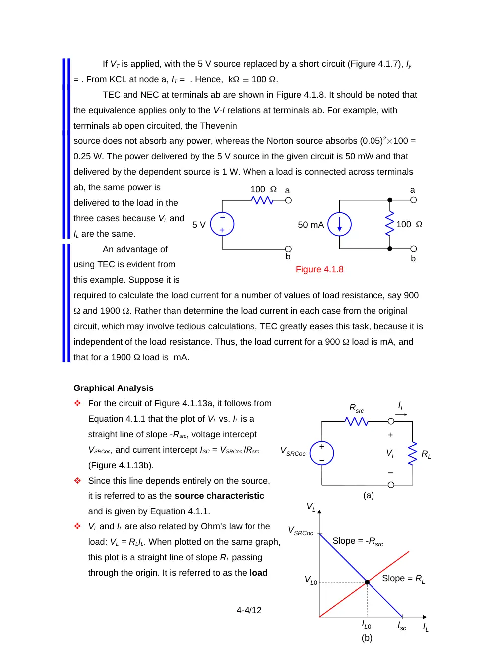TEC and NEC at terminals ab are shown in Figure 4.1.8. It should be noted that the equivalence applies only to the V-I relations at terminals ab. For example, with terminals ab open circuited, the Thevenin source does not absorb any power, whereas the Norton source absorbs (0.05)2100 = 0.25 W. The power delivered by the 5 V source in the given circuit is 50 mW and that delivered by the dependent source is 1 W. When a load is connected across terminals ab, the same power is delivered to the load in the three cases because VL and IL are the same. An advantage of using TEC is evident from this example. Suppose it is required to calculate the load current for a number of values of load resistance, say 900  and 1900 . Rather than determine the load current in each case from the original circuit, which may involve tedious calculations, TEC greatly eases this task, because it is independent of the load resistance. Thus, the load current for a 900  load is mA, and that for a 1900  load is mA. Graphical Analysis  For the circuit of Figure 4.1.13a, it follows from Equation 4.1.1 that the plot of VL vs. IL is a straight line of slope -Rsrc, voltage intercept VSRCoc, and current intercept ISC = VSRCoc /Rsrc (Figure 4.1.13b).  Since this line depends entirely on the source, it is referred to as the source characteristic and is given by Equation 4.1.1.  VL and IL are also related by Ohm’s law for the load: VL = RLIL. When plotted on the same graph, this plot is a straight line of slope RL passing through the origin. It is referred to as the load 4-4/12 5 V 100  a b a b 50 mA – + 100  Figure 4.1.8 Rsrc – + + – VL VSRCoc IL RL (a) VL IL Isc Slope = -Rsrc VSRCoc (b) VL0 IL0 Slope = RL line.  The intersection point of the load line and the source characteristic gives VL0 and IL0 for particular values of VSRCoc, Rsrc, and RL. This is because both the source characteristic and the load line equation are satisfied at the intersection point. 4.2 Substitution Theorem Statement An unknown resistor having a voltage V across it, or a current I through it, may be replaced by an ideal, independent voltage source V, or an ideal, independent current source I, without disturbing the rest of the circuit. 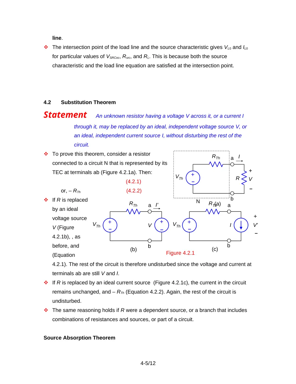 To prove this theorem, consider a resistor connected to a circuit N that is represented by its TEC at terminals ab (Figure 4.2.1a). Then: (4.2.1) or, – RTh (4.2.2)  If R is replaced by an ideal voltage source V (Figure 4.2.1b), , as before, and (Equation 4.2.1). The rest of the circuit is therefore undisturbed since the voltage and current at terminals ab are still V and I.  If R is replaced by an ideal current source (Figure 4.2.1c), the current in the circuit remains unchanged, and – RTh (Equation 4.2.2). Again, the rest of the circuit is undisturbed.  The same reasoning holds if R were a dependent source, or a branch that includes combinations of resistances and sources, or part of a circuit. Source Absorption Theorem 4-5/12 (a) V – + N – + VTh RTh a b R I Figure 4.2.1 (b) I' a b V – + (c) I a b – + V' – + VTh RTh – + VTh RTh  This is a weaker form of the substitution theorem, which may be stated as follows: Statement A resistor of known value having a voltage V across it AND a current I through it, may be replaced by a CCVS having V = RI, or a VCCS having I = V/ R. Conversely, a CCVS having V = I may be replaced by a resistance , and a VCCS having I = V may be replaced by a conductance , where V is the voltage across the source and I is the current through it. 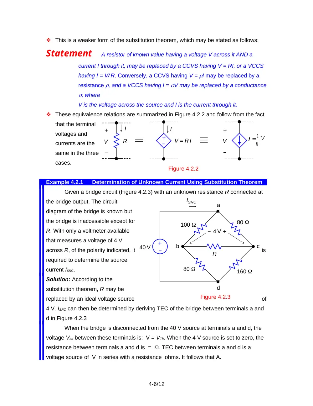 These equivalence relations are summarized in Figure 4.2.2 and follow from the fact that the terminal voltages and currents are the same in the three cases. Example 4.2.1 Determination of Unknown Current Using Substitution Theorem Given a bridge circuit (Figure 4.2.3) with an unknown resistance R connected at the bridge output. The circuit diagram of the bridge is known but the bridge is inaccessible except for R. With only a voltmeter available that measures a voltage of 4 V across R, of the polarity indicated, it is required to determine the source current ISRC. Solution: According to the substitution theorem, R may be replaced by an ideal voltage source of 4 V. ISRC can then be determined by deriving TEC of the bridge between terminals a and d in Figure 4.2.3 When the bridge is disconnected from the 40 V source at terminals a and d, the voltage Vad between these terminals is: V = VTh. When the 4 V source is set to zero, the resistance between terminals a and d is = . TEC between terminals a and d is a voltage source of V in series with a resistance ohms. It follows that A. 4-6/12 Figure 4.2.2 R + V + V I – – R I 1 V I + – V = R I – + – + a b 80  100  80  160  c d R 4 V 40 V ISRC Figure 4.2.3 4.3 Source Rearrangement Concept Sources may be rearranged in a circuit, so as to facilitate analysis of the circuit, without affecting circuit responses, as long as KCL and KVL remain satisfied. 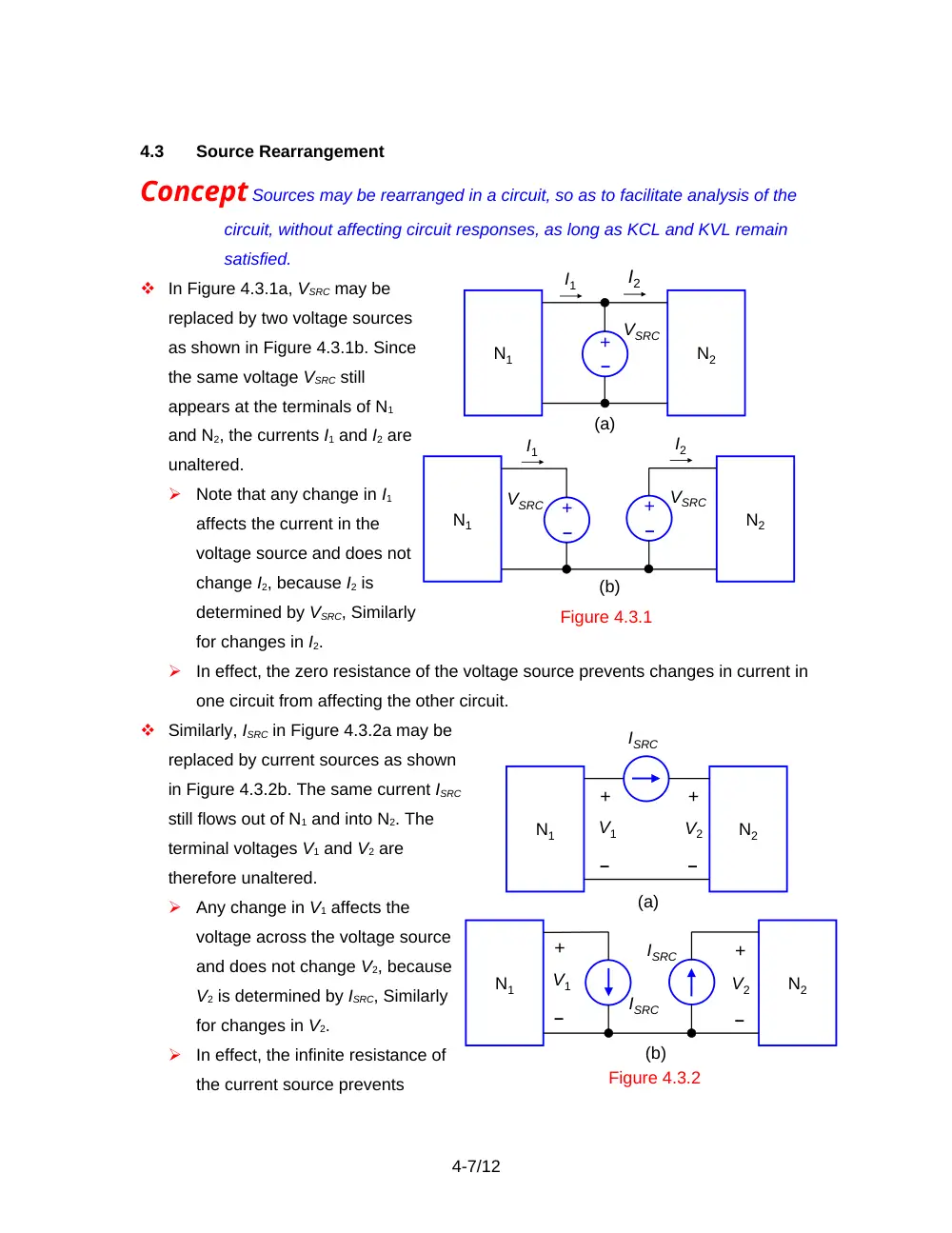 In Figure 4.3.1a, VSRC may be replaced by two voltage sources as shown in Figure 4.3.1b. Since the same voltage VSRC still appears at the terminals of N1 and N2, the currents I1 and I2 are unaltered.  Note that any change in I1 affects the current in the voltage source and does not change I2, because I2 is determined by VSRC, Similarly for changes in I2.  In effect, the zero resistance of the voltage source prevents changes in current in one circuit from affecting the other circuit.  Similarly, ISRC in Figure 4.3.2a may be replaced by current sources as shown in Figure 4.3.2b. The same current ISRC still flows out of N1 and into N2. The terminal voltages V1 and V2 are therefore unaltered.  Any change in V1 affects the voltage across the voltage source and does not change V2, because V2 is determined by ISRC, Similarly for changes in V2.  In effect, the infinite resistance of the current source prevents 4-7/12 Figure 4.3.1 N2 N1 VSRC I1 I2 – + (a) N2 N1 VSRC I1 I2 – + (b) VSRC – + Figure 4.3.2 N2 N1 ISRC (a) + – V2 + – V1 N2 N1 ISRC (b) ISRC + – V1 + – V2 changes in the voltage in one circuit from affecting the other circuit. Example 4.3.1 Source Rearrangement It is required to determine Ix in Figure 4.3.3 using source rearrangement. Solution: The voltage source and current source may each be split into two sources as shown in Figure 4.3.4. In Figure 4.3.3, a current of 10 A enters node b from the source and a current of 10 A leaves node a. The same conditions are preserved in Figure 4.3.4. A source current of 10 A both enters and leaves node c in Figure 4.3.4, so that the net source current at this node is zero, as in Figure 4.3.3. Ix will be determined in two ways: Method 1: The first method is to derive TEC between nodes b and a. The open-circuit voltages between nodes a and c, and between nodes b and c will be determined by superposition. When the 6  resistor is removed, and the A sources set to zero, V, and 4 V. Hence, nodes a and b will be at the same voltage, and this component of Vba is zero. If the 10 V sources are set to zero, V, and V. It follows that Vba = VTh = 36 V. With all sources set to zero, RTh = (4||6) + (2||3) = 3.6 . Hence A. Method 2: The second method is based on the substitution theorem and source transformation. The 6  resistor is replaced by a current source Ix, in accordance with the substitution theorem, which adds Ix to the two 10 A sources. The 10 V source on the RHS in Figure 4.3.4 is transformed to a 5/3 A current source. The parallel resistance of 6  and 4  is 12/5 , and . Similarly the 10 V source on the LHS in Figure 4.3.4 is transformed to 10/3 A current source in parallel with 6/5 ,and . From the circuit without the 6  resistor replaced by a current source, . 4-8/12 Figure 4.3.3 – + 10 V 3  6  4  2  6  10 A Ix a b Iy Figure 4.3.4 – + 10 V 3  6  4  2  6  Ix a b 10 A – + 10 V 10 A c Substituting gives A. 4.4 Removal of Redundant Elements Concept Redundant elements can be removed from a circuit without affecting the circuit responses of interest.  Examples of redundant elements are:  A resistor in series with an ideal current source. When this series resistor is removed, that is, replaced by a short circuit, the source current is unchanged. The voltage across the source decreases by an amount equal to the voltage drop across the resistor, but the rest of the circuit is not disturbed.  A resistor in parallel with an ideal voltage source. When this parallel resistor is removed, that is, replaced by an open circuit, the source voltage is unchanged. The current through the source decreases by an amount equal to the current through the resistor, but the rest of the circuit is not disturbed.  Resistors that do not carry any current. These may be replaced by an open circuit or a short circuit without disturbing the rest of the circuit.  Inductors and capacitors in a circuit under DC operating conditions. The inductor is replaced by a short circuit and the capacitor by an open circuit, as discussed in sections 1.8 and 1.9. 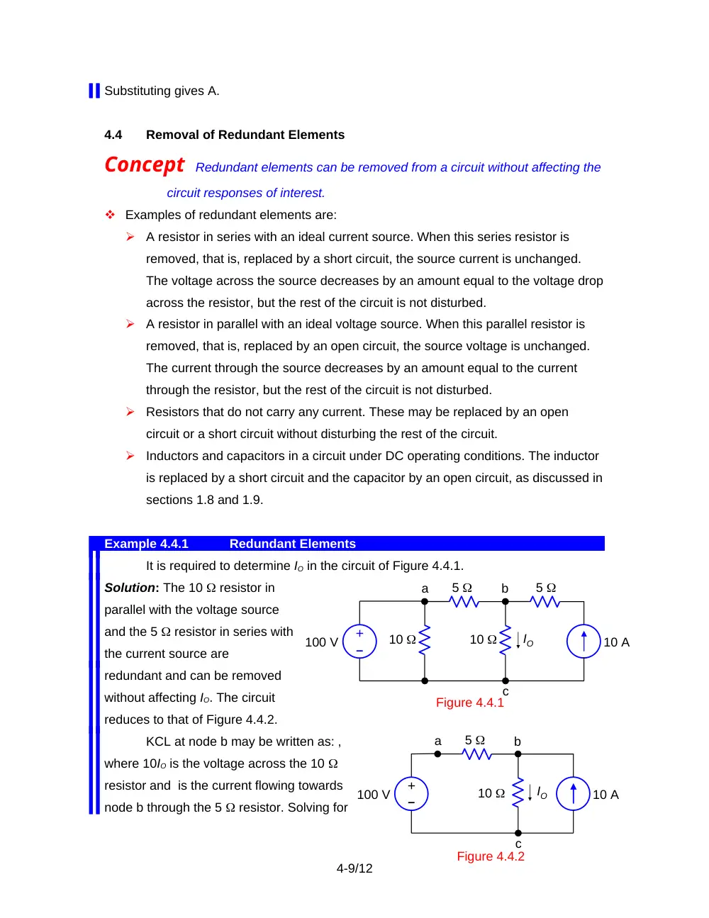Example 4.4.1 Redundant Elements It is required to determine IO in the circuit of Figure 4.4.1. Solution: The 10  resistor in parallel with the voltage source and the 5  resistor in series with the current source are redundant and can be removed without affecting IO. The circuit reduces to that of Figure 4.4.2. KCL at node b may be written as: , where 10IO is the voltage across the 10  resistor and is the current flowing towards node b through the 5  resistor. Solving for 4-9/12 5  Figure 4.4.1 100 V 10  10  10 A IO – + 5  a b c Figure 4.4.2 5  100 V 10  10 A IO – + a b c IO gives A. The two resistors do not affect IO. In Figure 4.4.2, the current through the voltage source is zero and the voltage across the current source is 100 V. In Figure 4.4.1, the current through the voltage source is 10 A, and the voltage across the current source is 150 V. 4.5 Exploitation of Symmetry Concept In circuits possessing symmetry, the circuit may be simplified by removing elements that do not carry current, or by connecting together nodes that are at the same voltage. 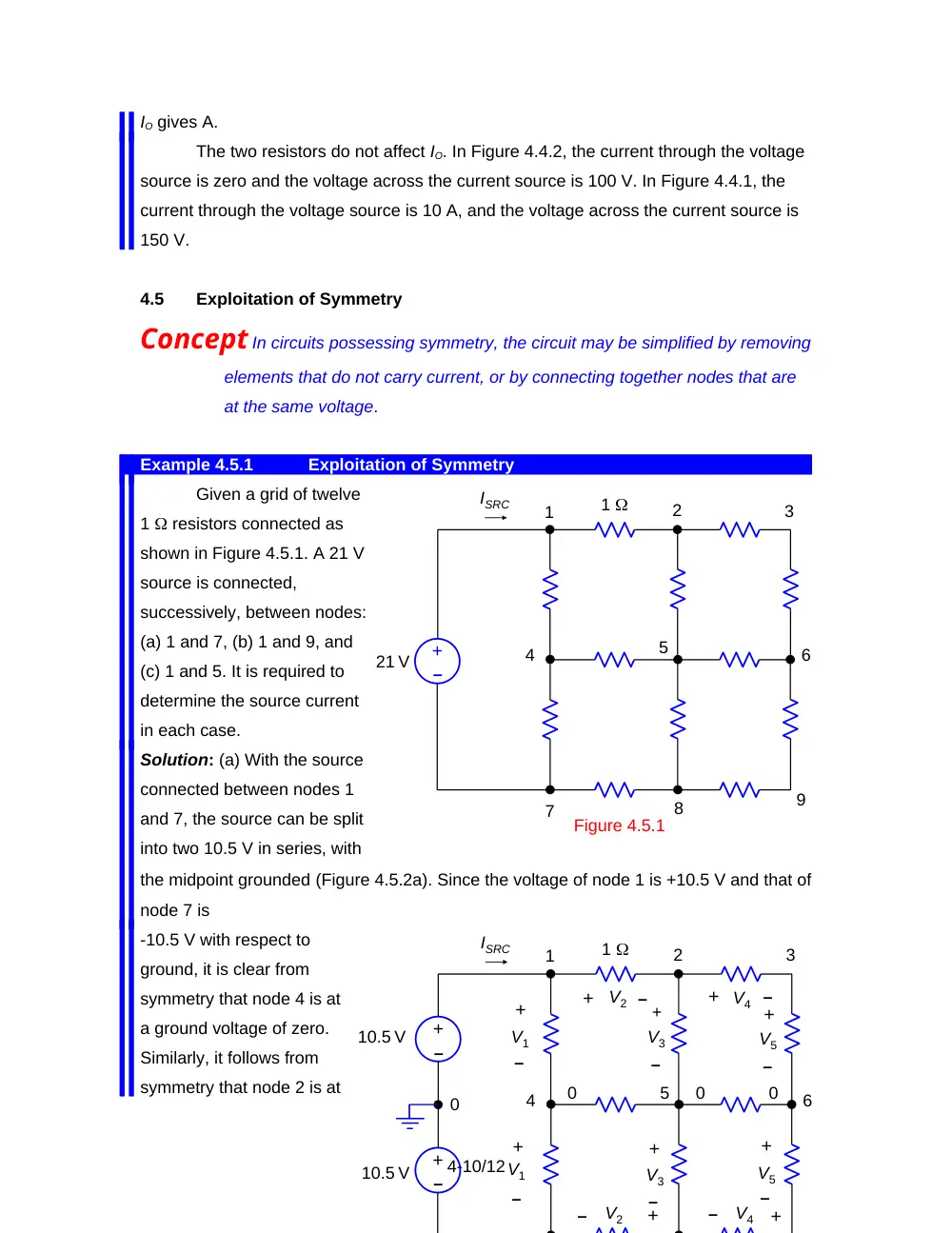Example 4.5.1 Exploitation of Symmetry Given a grid of twelve 1  resistors connected as shown in Figure 4.5.1. A 21 V source is connected, successively, between nodes: (a) 1 and 7, (b) 1 and 9, and (c) 1 and 5. It is required to determine the source current in each case. Solution: (a) With the source connected between nodes 1 and 7, the source can be split into two 10.5 V in series, with the midpoint grounded (Figure 4.5.2a). Since the voltage of node 1 is +10.5 V and that of node 7 is -10.5 V with respect to ground, it is clear from symmetry that node 4 is at a ground voltage of zero. Similarly, it follows from symmetry that node 2 is at 4-10/12 + – 1  21 V 1 2 3 4 5 6 7 8 9 ISRC Figure 4.5.1 + – 1  10.5 V 1 2 3 4 5 6 V2 V4 V1 V3 V5 V2 V4 V1 V3 V5 + – + – + – + – + – + – + – + – + – + – ISRC + – 10.5 V 0 0 0 0 a voltage 10.5 – V2, whereas node 8 is at -10.5 + V2, where V2 is a positive voltage drop. This means that the voltages of nodes 2 and 8 are equal in magnitude but opposite in sign. Node 5 is therefore at zero voltage. Since nodes 2 and 6 are connected by a resistance of 2 , as are nodes 6 and 8, then node 6 is also at a node voltage of zero. Hence, the resistors between nodes 4 and 5, and between nodes 5 and 6, do not carry any current. They could just as well be replaced by open circuits or short circuits. If they are replaced by open circuits, the circuit reduces to that shown in Figure 4.5.2b. The series-parallel combination of resistances evaluates to 1.25  across the source, so that ISRC = 16.8 A. Alternatively, it may be argued that the circuit of Figure 4.5.2a is symmetrical about a horizontal line passing through nodes 4, 5, 6, and the ground between the split sources. Voltages above this line are positive, whereas voltages below this line is negative. Hence, voltages along the line are zero. (b) If the 21 V source is connected between nodes 1 and 9 (Figure 4.5.1), the circuit becomes symmetrical about the diagonal and could be split into two halves alon the diagonal. Figure 4.5.3a shows the source applied to one hal-circuit. The half-circuit can be reduced to that shown in Figure 4.5.3b, from which it follows that the current drawn by the half circuit is 7 A, so that Isrc = 14 A. 4-11/12 + – 21 V 1 2 3 5 6 9 (a) + – 1  21 V 1 9 7 A 1  Figure 4.5.3 (b) 2 6 1  (c) When the 21 V source is connected between nodes 1 and 5 (Figure 4.5.4a), the currents are symmetrical about the diagonal through nodes 1, 5, and 9. Thus, the current from node 1 to node 2 equals that from node 1 to node 4, the current from node 3 to node 6 equals that from node 7 to node 8, and the current from node 6 to node 9 equals that from node 8 to node 9. The currents at node 9 are therefore equal and sum to zero. Hence, each of them must be zero. It follows that the two resistors connected to node 9 do not carry current and may be removed. The resulting circuit becomes as shown in Figure 4.5.5b. The resistance on either side of the source is 7/4 . The effective resistance across the source is 7/8 , so that ISRC = 24 A. 4-12/12 + – 1 2 3 4 5 6 7 8 9 21 V 0 0 (a) + – 1  21 V 1  1  3  3  1  Figure 4.5.4 (b)