EECE 210 Chapter 6, Fall 2012

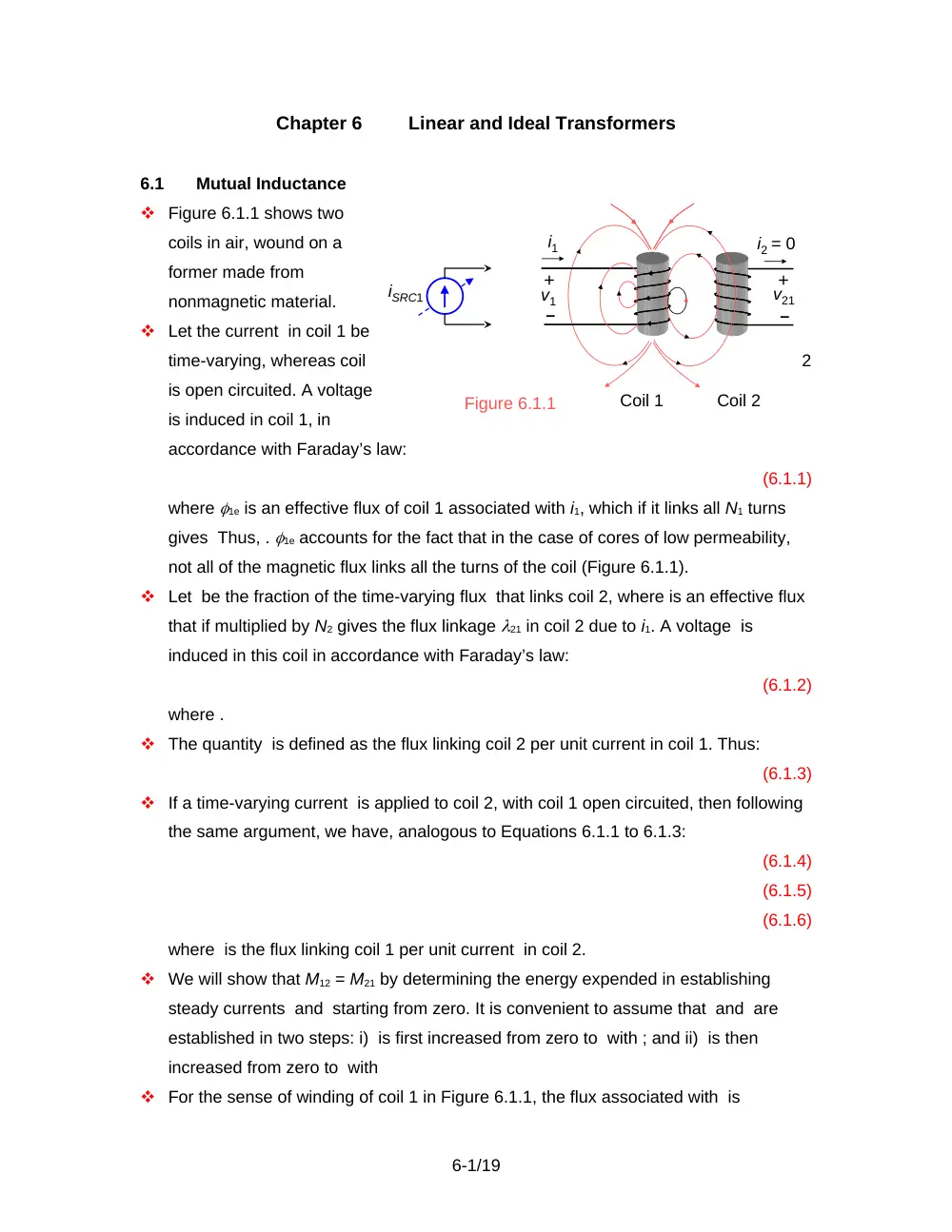
Chapter 6 Linear and Ideal Transformers 6.1 Mutual Inductance  Figure 6.1.1 shows two coils in air, wound on a former made from nonmagnetic material.  Let the current in coil 1 be time-varying, whereas coil 2 is open circuited. A voltage is induced in coil 1, in accordance with Faraday’s law: (6.1.1) where 1e is an effective flux of coil 1 associated with i1, which if it links all N1 turns gives Thus, . 1e accounts for the fact that in the case of cores of low permeability, not all of the magnetic flux links all the turns of the coil (Figure 6.1.1).  Let be the fraction of the time-varying flux that links coil 2, where is an effective flux that if multiplied by N2 gives the flux linkage 21 in coil 2 due to i1. A voltage is induced in this coil in accordance with Faraday’s law: (6.1.2) where .  The quantity is defined as the flux linking coil 2 per unit current in coil 1. Thus: (6.1.3)  If a time-varying current is applied to coil 2, with coil 1 open circuited, then following the same argument, we have, analogous to Equations 6.1.1 to 6.1.3: (6.1.4) (6.1.5) (6.1.6) where is the flux linking coil 1 per unit current in coil 2.  We will show that M12 = M21 by determining the energy expended in establishing steady currents and starting from zero. It is convenient to assume that and are established in two steps: i) is first increased from zero to with ; and ii) is then increased from zero to with  For the sense of winding of coil 1 in Figure 6.1.1, the flux associated with is 6-1/19 i1 + – v1 + – v21 i2 = 0 Figure 6.1.1 Coil 1 Coil 2 iSRC1 downward in this coil, according to the right-hand rule. While is increasing, the induced voltage = in coil 1 opposes the increase in in accordance with Lenz’s law, by being a voltage drop across L1 in the direction of i1. 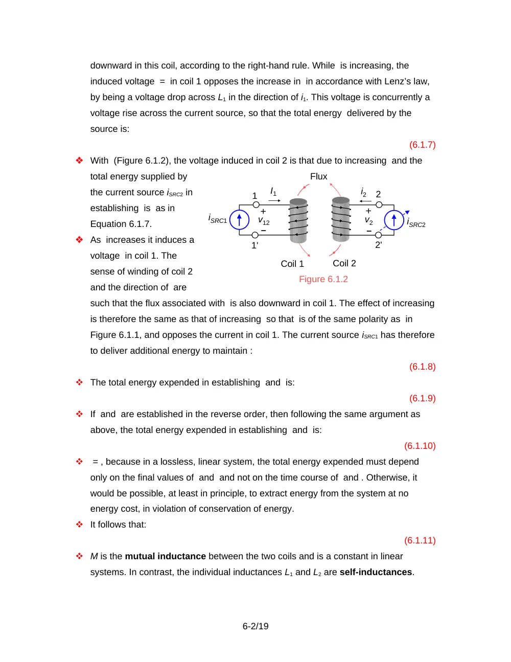This voltage is concurrently a voltage rise across the current source, so that the total energy delivered by the source is: (6.1.7)  With (Figure 6.1.2), the voltage induced in coil 2 is that due to increasing and the total energy supplied by the current source iSRC2 in establishing is as in Equation 6.1.7.  As increases it induces a voltage in coil 1. The sense of winding of coil 2 and the direction of are such that the flux associated with is also downward in coil 1. The effect of increasing is therefore the same as that of increasing so that is of the same polarity as in Figure 6.1.1, and opposes the current in coil 1. The current source iSRC1 has therefore to deliver additional energy to maintain : (6.1.8)  The total energy expended in establishing and is: (6.1.9)  If and are established in the reverse order, then following the same argument as above, the total energy expended in establishing and is: (6.1.10)  = , because in a lossless, linear system, the total energy expended must depend only on the final values of and and not on the time course of and . Otherwise, it would be possible, at least in principle, to extract energy from the system at no energy cost, in violation of conservation of energy.  It follows that: (6.1.11)  M is the mutual inductance between the two coils and is a constant in linear systems. In contrast, the individual inductances L1 and L2 are self-inductances. 6-2/19 Figure 6.1.2 I1 + – v12 + – v2 i2 Coil 1 Coil 2 Flux iSRC2 1 1' 2 2' iSRC1 Definition The mutual inductance of two magnetically-coupled coils is the flux linkage in one coil per unit current in the other coil. It is independent of which coil carries the current.  If either the polarity of iSRC2, or the sense of winding of coil 2, is reversed in Figure 6.1.2, the flux due to becomes upward in coil 1. The polarity of is reversed and becomes a voltage drop across the current source iSRC1. Energy is therefore returned to the source and the sign of the energy term involving becomes negative in Equations 6.1.9 and 6.1.10. M, however, is always a positive quantity. 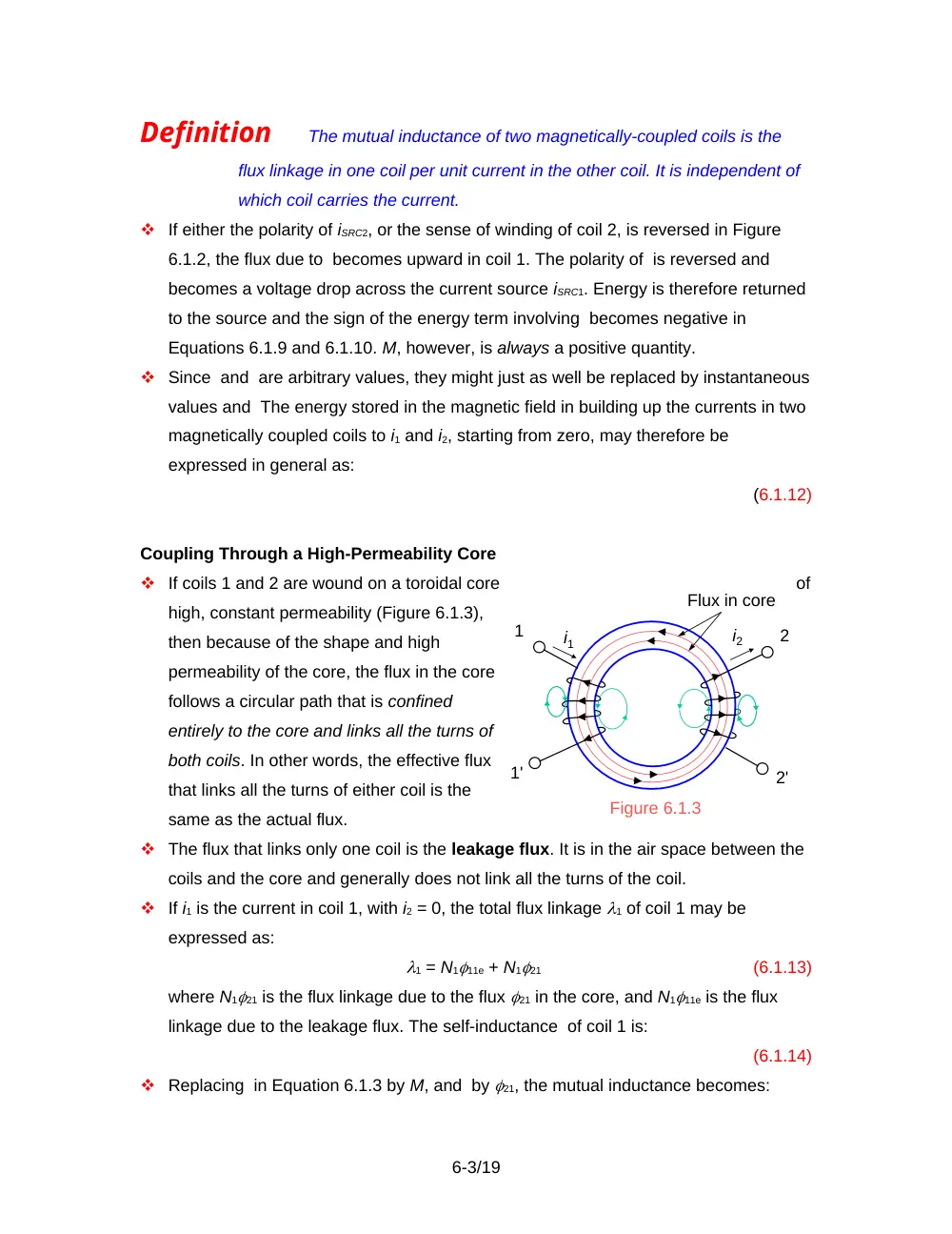 Since and are arbitrary values, they might just as well be replaced by instantaneous values and The energy stored in the magnetic field in building up the currents in two magnetically coupled coils to i1 and i2, starting from zero, may therefore be expressed in general as: (6.1.12) Coupling Through a High-Permeability Core  If coils 1 and 2 are wound on a toroidal core of high, constant permeability (Figure 6.1.3), then because of the shape and high permeability of the core, the flux in the core follows a circular path that is confined entirely to the core and links all the turns of both coils. In other words, the effective flux that links all the turns of either coil is the same as the actual flux.  The flux that links only one coil is the leakage flux. It is in the air space between the coils and the core and generally does not link all the turns of the coil.  If i1 is the current in coil 1, with i2 = 0, the total flux linkage 1 of coil 1 may be expressed as: 1 = N111e + N121 (6.1.13) where N121 is the flux linkage due to the flux 21 in the core, and N111e is the flux linkage due to the leakage flux. The self-inductance of coil 1 is: (6.1.14)  Replacing in Equation 6.1.3 by M, and by 21, the mutual inductance becomes: 6-3/19 Figure 6.1.3 i1 1' 1 Flux in core i2 2' 2 (6.1.15)  If i2 is the current in coil 2, with i1 = 0, the relations corresponding to Equations 6.1.13 to 6.1.15 are obtained by repeating the above arguments. Thus: 2 = N222e + N212 (6.1.16) (6.1.17) (6.1.18) Coupling Coefficient  Multiplying together Equations 6.1.15 and 6.1.18: (6.1.19) Dividing by the product L1L2 from Equations 6.1.14 and 6.1.17: (6.1.20)  The expression is a measure of how effectively coil 1 is coupled to the core. Similarly for . The product on the RHS of Equation 6.1.20 is a measure of how well the two coils are magnetically coupled together through the core.  Equation 6.1.20 may be written as: or (6.1.21) Definition The coupling coefficient k of two magnetically-coupled coils is defined as and is a measure of how tightly the two coils are coupled through the core. It assumes values in the range of 0 to unity, where k = 0 denotes no coupling and k = 1 denotes perfect coupling. Electric Circuit Analogy  A useful analogy can be made between a magnetic systems and electric circuits (Table 6.1.1).  Magnetic flux is analogous to electric current, and 6-4/19 Table 6.1.1 Electric Circuit Analogy Electric Circuit Magnetic System Current Flux () Voltage excitation (emf) mmf (Ni) Resistance Reluctance (mmf/flux) Conductance Permeance (flux/mmf) Conductivity Permeability magnetomotive force (mmf), which equals Ni and drives magnetic flux, is analogous to voltage excitation, also known as electromotive force (emf). Flux is the product of permeance and mmf. 6.2 The Linear Transformer Definition A transformer consists of two or more coils that are magnetically coupled relatively tightly. In a linear transformer, permeability is constant, so that B and H, or  and i, are linearly related. 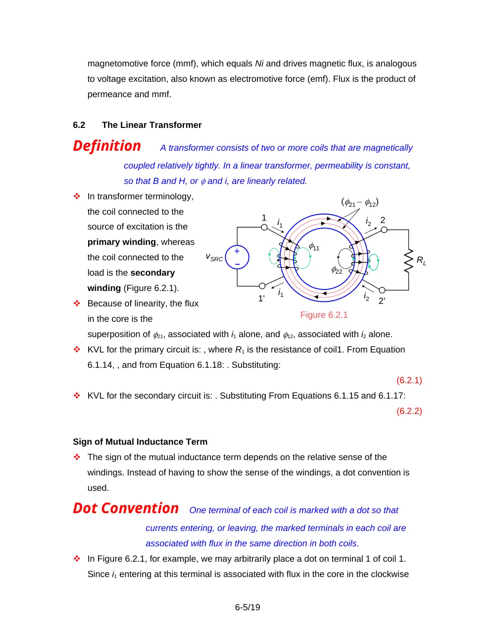 In transformer terminology, the coil connected to the source of excitation is the primary winding, whereas the coil connected to the load is the secondary winding (Figure 6.2.1).  Because of linearity, the flux in the core is the superposition of 21, associated with i1 alone, and 12, associated with i2 alone.  KVL for the primary circuit is: , where R1 is the resistance of coil1. From Equation 6.1.14, , and from Equation 6.1.18: . Substituting: (6.2.1)  KVL for the secondary circuit is: . Substituting From Equations 6.1.15 and 6.1.17: (6.2.2) Sign of Mutual Inductance Term  The sign of the mutual inductance term depends on the relative sense of the windings. Instead of having to show the sense of the windings, a dot convention is used. Dot Convention One terminal of each coil is marked with a dot so that currents entering, or leaving, the marked terminals in each coil are associated with flux in the same direction in both coils.  In Figure 6.2.1, for example, we may arbitrarily place a dot on terminal 1 of coil 1. Since i1 entering at this terminal is associated with flux in the core in the clockwise 6-5/19 Figure 6.2.1 – + vSRC RL i1 i2 i1 1' 1 (21 – 12) i2 2' 2 11 22 direction, and i2 entering terminal 2 is also associated with flux in the same direction, terminal 2 is dotted. Alternatively, terminals 1 and 2 may be dotted. If the sense of winding of either coil is reversed, as in Figure 6.1.3, then the dotted terminals will be 1 and 2, or 1 and 2. In Figure 6.1.2, terminals 1 and 2, or 1 and 2, will be dotted.  An alternative interpretation of the dot markings, which follows from the above, is that the polarities of induced voltages in both coils are the same, relative to the dot markings. In Figure 6.1.2, when i2 is increasing, v2 opposes the increase in i2 and v12 opposes I1. Both voltages oppose currents entering at the dotted terminals, and the polarities of these voltages make the dotted terminal positive with respect to the unmarked terminal in both coils.  Once the terminals are marked with dots, the sign of the M term readily follows: Sign of M Term If the assigned positive directions of currents are such that these currents both flow in, or both flow out, at the dotted terminals, the sign of the mutual inductance term (Mdi1 /dt, or Mdi2 /dt) for either coil is the same as that of the self-inductance term for that coil (L1di1 /dt, or L2di2 /dt) . Otherwise, the sign of the mutual inductance term for either coil is opposite that of the self-inductance term for that coil.  The justification is that if the assigned positive directions of coil currents are such that both currents flow into, or out of, the dotted terminals, and produce flux in the same direction in the core. This means that the voltage induced by in coil 1 is of the same polarity as the voltage induced by in coil 1, so that these two terms have the same sign in the voltage relations of coil 1. Similarly for the voltage induced by in coil 2 and the term. 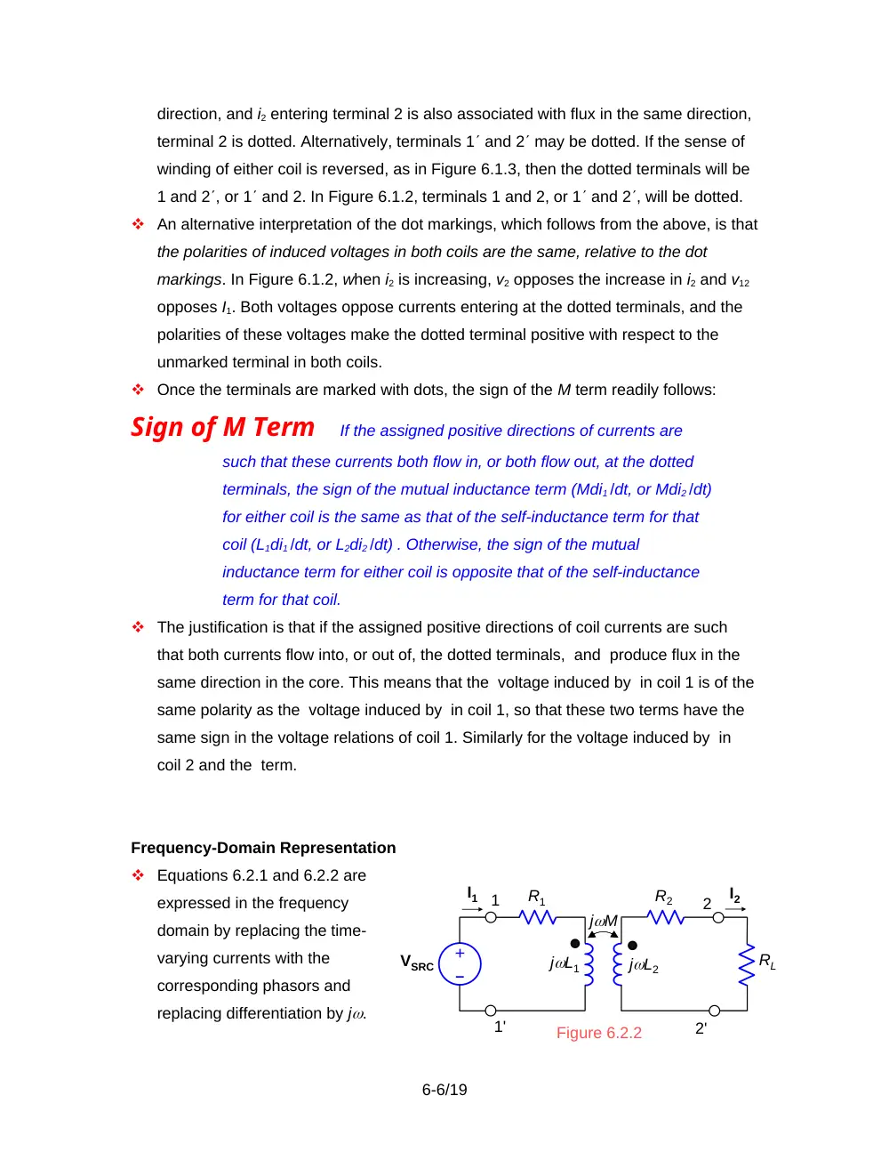Frequency-Domain Representation  Equations 6.2.1 and 6.2.2 are expressed in the frequency domain by replacing the time- varying currents with the corresponding phasors and replacing differentiation by j. 6-6/19 Figure 6.2.2 I2 VSRC I1 – + RL jL2 jL1 jM R2 R1 1' 1 2' 2 (Figure 6.2.2). 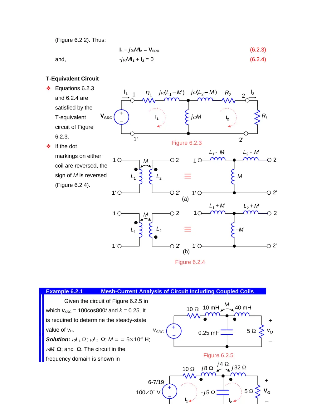Thus: I1 – jMI2 = VSRC (6.2.3) and, -jMI1 + I2 = 0 (6.2.4) T-Equivalent Circuit  Equations 6.2.3 and 6.2.4 are satisfied by the T-equivalent circuit of Figure 6.2.3.  If the dot markings on either coil are reversed, the sign of M is reversed (Figure 6.2.4). Example 6.2.1 Mesh-Current Analysis of Circuit Including Coupled Coils Given the circuit of Figure 6.2.5 in which vSRC = 100cos800t and k = 0.25. It is required to determine the steady-state value of vO. Solution: L1 ; L2 ; M   510-3 H; M ; and . The circuit in the frequency domain is shown in 6-7/19 Figure 6.2.3 I2 VSRC I1 – + RL jM R2 R1 1' 1 2' 2 j(L1 – M ) j(L2 – M ) I2 I1 Figure 6.2.4 M 1' 1 2' 2 L1  M L2  M - M 1' 1 2' 2 L1 + M L2 + M L2 L1 M 1' 1 2' 2 L2 L1 M 1' 1 2' 2   (a) (b) 10  M + _ vO 0.25 mF vSRC Figure 6.2.5 – + 10 mH 40 mH 5  10  + _ VO 1000 V – + j 8  5  j 4  j 32  - j 5  I2 I1 Figure 6.2.6. In writing the mesh current equation for mesh 1, the total voltage drop in this mesh due to I1 equals, as usual, I1 multiplied by the total self-impedance of this mesh, that is,(10 + j8 – j5)I1. I2 introduces as usual a voltage rise of ZcI2 in mesh 1, where Zc =- j5  is the common impedance between meshes 1 and 2, plus a jMI2 term due to the magnetic coupling between the coils in the two meshes. Since both I1 and I2 enter at the dotted terminals, the sign of the jMI2 term is the same as that of jL1 term in the equation of mesh 1 and the same as that of the jL2 term in the equation for mesh 2. The mesh-current equation for mesh 1 is therefore: (6.2.5) Similarly, the mesh-current equation for mesh 2 is: (6.2.6) Solving for I2 gives: I2 = - 3.0636 – j0.5375 A, so that VO = 5I2 = -15.3 – j2.69 = 15.55-170.0 V, or vO = 15.55cos(800t – 170.0) V. Equations 6.2.5 and 6.2.6 could just as well be derived using the T-equivalent circuit (Figure 6.2.7). If L1 in Figure 6.2.6a is rotated clockwise and L2 is rotated counterclockwise so as to bring them to the upright position, the dot markings will be as in the transformer of Figure 6.2.4b. The appropriate T-equivalent circuit is therefore that having series branches L1 + M and L2 + M and a shunt branch –M. If the assigned positive direction of I2 in Figure 6.2.4 is made counterclockwise, and this current is denoted by then flows into the unmarked terminal of coil 2. The sign of the mutual inductance term is now opposite that of the self-inductance term for each coil. The Zc term in the mutual impedance between the two meshes becomes positive since the voltage drop due to flowing in Zc is also a voltage drop in mesh 1. Equations 6.2.5 and 6.2.6 become: (6.2.7) and, (6.2.8) Now = – I2 and Vo = –R2= R2I2 as before. The T-equivalent circuit is the same as in Figure 6.4.6b. 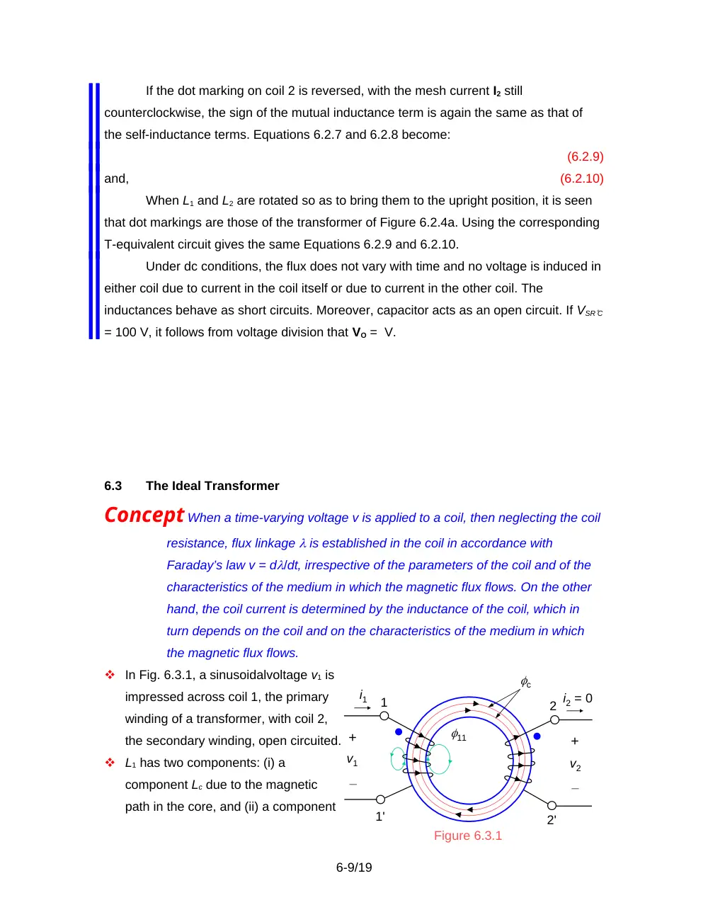6-8/19 Figure 6.2.7 10  + _ VO 1000 V – + j 12  5  j 36  - j 5  I2 I1 - j 4  If the dot marking on coil 2 is reversed, with the mesh current I2 still counterclockwise, the sign of the mutual inductance term is again the same as that of the self-inductance terms. Equations 6.2.7 and 6.2.8 become: (6.2.9) and, (6.2.10) When L1 and L2 are rotated so as to bring them to the upright position, it is seen that dot markings are those of the transformer of Figure 6.2.4a. Using the corresponding T-equivalent circuit gives the same Equations 6.2.9 and 6.2.10. Under dc conditions, the flux does not vary with time and no voltage is induced in either coil due to current in the coil itself or due to current in the other coil. The inductances behave as short circuits. Moreover, capacitor acts as an open circuit. If VSRC = 100 V, it follows from voltage division that VO = V. 6.3 The Ideal Transformer Concept When a time-varying voltage v is applied to a coil, then neglecting the coil resistance, flux linkage  is established in the coil in accordance with Faraday’s law v = d/dt, irrespective of the parameters of the coil and of the characteristics of the medium in which the magnetic flux flows. On the other hand, the coil current is determined by the inductance of the coil, which in turn depends on the coil and on the characteristics of the medium in which the magnetic flux flows. 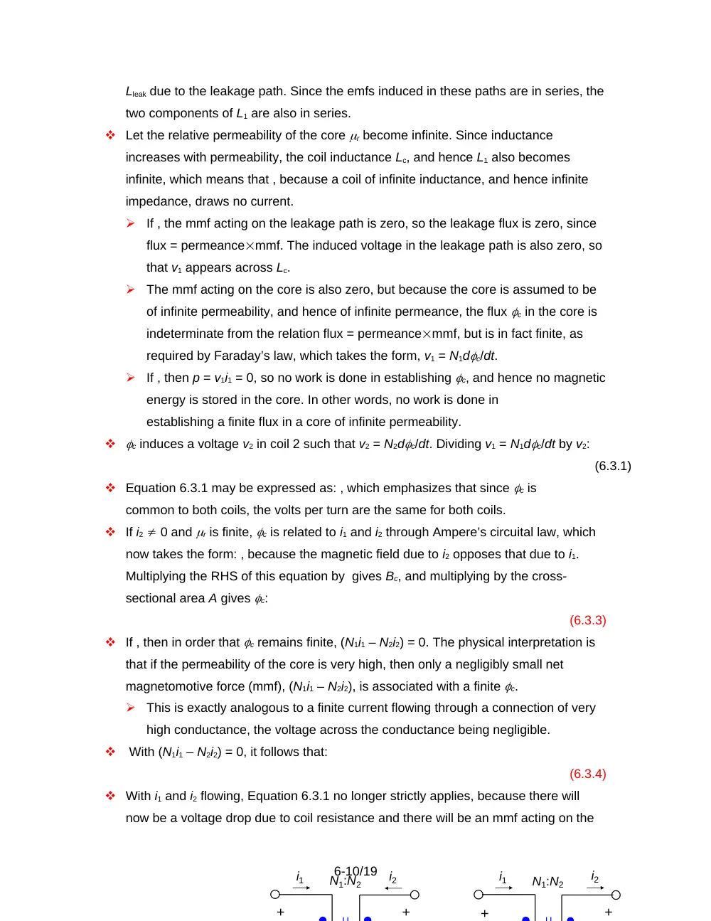 In Fig. 6.3.1, a sinusoidalvoltage v1 is impressed across coil 1, the primary winding of a transformer, with coil 2, the secondary winding, open circuited.  L1 has two components: (i) a component Lc due to the magnetic path in the core, and (ii) a component 6-9/19 Figure 6.3.1 v1 i1 1' 1 c 2' 2 11 i2 = 0 + _ + _ v2 Lleak due to the leakage path. Since the emfs induced in these paths are in series, the two components of L1 are also in series.  Let the relative permeability of the core r become infinite. Since inductance increases with permeability, the coil inductance Lc, and hence L1 also becomes infinite, which means that , because a coil of infinite inductance, and hence infinite impedance, draws no current.  If , the mmf acting on the leakage path is zero, so the leakage flux is zero, since flux = permeancemmf. The induced voltage in the leakage path is also zero, so that v1 appears across Lc.  The mmf acting on the core is also zero, but because the core is assumed to be of infinite permeability, and hence of infinite permeance, the flux c in the core is indeterminate from the relation flux = permeancemmf, but is in fact finite, as required by Faraday’s law, which takes the form, v1 = N1dc/dt.  If , then p = v1i1 = 0, so no work is done in establishing c, and hence no magnetic energy is stored in the core. In other words, no work is done in establishing a finite flux in a core of infinite permeability.  c induces a voltage v2 in coil 2 such that v2 = N2dc/dt. Dividing v1 = N1dc/dt by v2: (6.3.1)  Equation 6.3.1 may be expressed as: , which emphasizes that since c is common to both coils, the volts per turn are the same for both coils.  If i2  0 and r is finite, c is related to i1 and i2 through Ampere’s circuital law, which now takes the form: , because the magnetic field due to i2 opposes that due to i1. Multiplying the RHS of this equation by gives Bc, and multiplying by the cross- sectional area A gives c: (6.3.3)  If , then in order that c remains finite, (N1i1 – N2i2) = 0. The physical interpretation is that if the permeability of the core is very high, then only a negligibly small net magnetomotive force (mmf), (N1i1 – N2i2), is associated with a finite c.  This is exactly analogous to a finite current flowing through a connection of very high conductance, the voltage across the conductance being negligible.  With (N1i1 – N2i2) = 0, it follows that: (6.3.4)  With i1 and i2 flowing, Equation 6.3.1 no longer strictly applies, because there will now be a voltage drop due to coil resistance and there will be an mmf acting on the 6-10/19 i1 i2 + + i1 i2 + + N1:N2 N1:N2 leakage path to produce a leakage flux and hence a voltage drop. Thus, in order that both Equations 6.3.1 and 6.3.4 apply, we have to assume negligible resistance and perfect coupling between the coils and the core.  If the assigned positive direction of and do not conform to the dot markings . Similarly, if and both enter or leave at the dotted terminals, so that . The four possibilities are illustrated in Figure 6.3.2.  It follows from the voltage and current ratios that the instantaneous power input equals the instantaneous power output, neglecting power losses in the core. Definition An ideal transformer is a two-port device that neither dissipates nor stores energy, and whose input-output v-i relations are of the form: and  From Equation 1.9.8: and , so that: (6.3.5) independently of r. Thus, although each of L1 and L2 becomes infinite as r becomes infinite, their ratio remains finite and equal to the square of the turns ratio. Phasor Relations  Figure 6.3.3b shows the phasor diagram for the ideal transformer of Figure 6.3.3a. Figure 6.3.3c is a flow diagram of the causal relationships.  A voltage V1 applied to the primary winding establishes a flux c in the core such that c V1 and lags V1 by 90. c induces a voltage V2 in the secondary winding such that V2c, assuming the assigned positive directions and dot markings shown. Since V2 leads c by 90, it is in phase with V1. V2 causes a current I2 in the secondary circuit, which lags V2 by an angle , assuming ZL is inductive. In order to have zero mmf in 6-11/19 2 1 2 1 N N v v   1 2 2 1 N N i i  2 1 2 1 N N v v   1 2 2 1 N N i i   (c) (d) Figure 6.3.2 i1 i2 v2 _ + v1 _ + i1 i2 v2 _ + v1 _ + N1:N2 N1:N2 V1 1/jN1 c jN2 1/ZL V1 ZL + _ V2 _ + I1 I2 V1 V2 I2 I1 c  (a) (b) (c) N1:N2 N1I1 – N2I2 = 0 I2 V2 I1 the core, a current I1 flows in the primary winding such that I1I2. Reflected Impedance  For the dot markings and assigned positive directions of Figure 6.3.3a: and . Dividing these two equations: . Substituting : (6.3.6)  Because of squaring of the turns ratio, Equation 6.3.6 is valid for any of the configurations of Figure 6.3.3a to d.  An open circuit is reflected as an open circuit, and a short circuit is reflected as a short circuit. Example 6.3.1 Ideal Transformer Circuit Assume that in Figure 6.3.4, v1 = 120cos1000t, N1:N2 = 1:2, and that Z consists of a resistance of 10  in series with a 20 mH inductor. It is required to determine the primary current and the secondary current and voltage. Solution: V2 = V1 = 2400 V; hence I2 = -63.4 A. It follows that I1 = I2 -63.4 A. The Ideal Autotransformer  Consider a two-winding transformer having (Figure 6.3.5a). v1 can be stepped up to v2 by adding to v1 a voltage , resulting in a step-up autotransformer (Figure 6.3.5b).  A winding of is required, and the current in the common winding is i1 – i2, which means that this winding can have a conductor of smaller cross- sectional area. Both of these considerations make the autotransformer smaller and lighter. In addition, terminal a in Figure 6.3.5b 6-12/19 V1 + _ V2 _ + I1 I2 Figure 6.3.4 N1:N2 10  j 20  i1 i2 + _ v2 Load c v1 (a) N1 N2 + _ d a b 2 N 1 N i1 – i2 i2 + _ + _ v2 Load a b d i1 (b) Figure 6.3.5 v1 + _ 2 v  could be connected to a slider over a bare part of the winding, so that a variable turns ratio is obtained.  The principal disadvantage of the autotransformer is that the input and output sides are not electrically isolated, because of the conduction path between them.  The voltage and current relations for the autotransformer follow directly from those of the two-winding transformer by substituting . Thus: (6.3.8) (6.3.9)  If the dot marking on either winding is reversed, the effective turns ratio becomes . Example 6.3.2 Three-Winding Transformer Given a three-winding ideal transformer with loads Z2 and Z3 connected as shown in Figure 6.3.7. It is required to determine the input impedance. Solution: Method 1: Since the voltage induced per turn is the same for all windings, , and , where the assigned positive directions of V1, V2, and V3 are all in accordance with the dots, so that the volts per turn are positive for all the windings. Since the net mmf in the core must be zero, = 0, where and . Note that I1 and (I1 – I2) enter at the dotted terminals of their respective windings. Their mmfs are in the same sense and may be assigned a positive sign. I3 leaves its winding at the dotted terminals, so its mmf is assigned a negative sign. Eliminating , , , and from these equations gives: (6.3.10) If , the impedance reflected to the primary side is , as for a two-winding transformer of turns ratio . If , the reflected impedance is , as for an autotransformer of turns N1 and N2. In fact, these reflected impedances in parallel give the reflected impedance of Equation 6.3.10. 6-13/19 + Z2 I2 I1 I3 Z3 + V3 N2 I1  I2 + V1 V2 Figure 6.3.7 1 N _ _ N3 _ Method 2: Let the impedances be replaced by current sources I2 and I3, in accordance with the substitution theorem, as shown in Figure 6.3.8, where and . We now apply superposition. If is applied alone, the primary current is . If is applied alone, the primary current is . With both sources applied, the primary current is I1 = + . Substituting for the currents in terms of voltages and impedances: I1 = + . But = V1 and =V1. Substituting for and gives: I1 = V1. The reflected impedance V1 / I1 is the same as that obtained above. Note that superposition strictly applies to voltage sources and current sources only. It cannot be applied directly to impedances, such as Z2 and Z3 in this Example. However, the substitution theorem allowed us to apply superposition after replacing these impedances with sources. 6.4 Reflection of Circuits Concept Circuits involving ideal transformers can be conveniently analyzed by reflecting the circuit on the primary side to the secondary side, or conversely.  Consider Figure 6.4.1. KCL for node q is: I2 + IL(V2 – Vy) (6.4.1) 6-14/19 _ + + _ VSRC Vy + _ V1 V2 I1 I2 ISRC Ix IL Zsrc ZL p q 1:a Primary side Secondary side + _ Figure 6.4.1 I2 I1 I3 + V3 N2 + V1 V2 Figure 6.3.8 _ N3 _ – + N1  Substituting: V2 = aV1 and I2I1, Equation 6.4.1 may be expressed as: I1IL (6.4.2) where .  This is KCL for a node q′ in Figure 6.4.2. The voltage V1 at node p and the current I1 leaving this node, are unaltered. The ideal transformer now appears at the extreme right with its secondary open-circuited. Since it is not serving any useful function, it can be omitted from the circuit.  In Figure 6.4.2, the secondary circuit is reflected to the primary side, element by element. If a > 1, voltages are stepped down by a and currents are stepped up by a. Impedances are stepped down, like voltages, but by a factor a2.  In a similar manner, we may write KCL for node p in Figure 6.4.1 as: (6.4.3)  Substituting: and , Equation 6.4.3 may be expressed as: (6.4.4) where . This is KCL for a node p′ on the secondary side in Figure 6.4.3. The voltage and currents at node q are unaltered. The ideal transformer now appears at the extreme left of the figure with its primary open- circuited. Since it is not serving any useful function, it can be omitted from the circuit.  In reflecting circuits from one side to the other, the order of the elements, left to right or right to left, must be preserved. Otherwise, the circuit is altered.  Controlling currents or voltages of dependent sources are reflected like any other voltage or current. 6-15/19 aVSRC Vy + V2 I2 ISRC /a Ix /a IL a2Zsrc p q ZL 1:a + _ + _ _ Figure 6.4.3 VSRC Vy /a + V1 I1 ISRC Ix aIL Zsrc p q 1:a 2 a Z L + _ + _ _ Figure 6.4.2  When the dot markings are reversed, a negative value of a is used. 6.5 Transformer Imperfections  Practical transformers depart from the ideal in the following respects:  finite inductance of the windings;  finite leakage flux;  power losses, because of finite resistance of the windings and core losses;  capacitances between primary and secondary windings as well as between layers of the same winding. The capacitances arise because of voltage differences and consequent energy storage in the electric field.  The finite resistances of the windings are accounted for, at least at low frequencies, by adding them at the terminals of the respective winding  The distributed capacitance between windings and layers of the same winding are accounted for in an approximate manner by lumped capacitances connected across the terminals of the primary and secondary windings and between these windings.  Ignoring the aforementioned imperfections, except for finite inductances and imperfect coupling, we are left with a linear transformer consisting of two coupled, lossless coils, of inductances L1 and L2 (Figure 6.5.1).  The governing equations are Equations 6.2.3 and 6.2.4, with R1 = 0 = R2, and with RL replaced by ZL: I1 – jMI2 = VSRC (6.5.1) -jMI1 + I2 = 0 (6.5.2)  Any circuit that represents the effect of finite inductances of windings and finite leakage fluxes must satisfy these equations. Finite Inductance of Windings  Let the coils to be perfectly coupled to begin with, that is, . Substituting for I2 from Equation 6.5.2 in Equation 6.5.1: (6.5.3)  With , it follows that the impedance seen by the source is that of jL2 in parallel with ZL, reflected to the primary 6-16/19 I2 I1 I2 VSRC I1 – + Inductance ratio L1:L2 (a) jL2 1' 1 2' 2 ZL Figure 6.5.1 I2 VSRC I1 – + ZL jL2 jL1 jM 1' 1 2' 2 side of an ideal transformer having an inductance ratio of L1:L2, or a turns ratio (Equation 6.3.5), as illustrated in Figure 6.5.2a. The impedance jL2 reflected to the primary side becomes jL1 (Figure 6.5.2b).  It is seen that the effect of finite inductances of an otherwise ideal transformer is to introduce a shunt impedance jL1 on the primary side, or a shunt impedance jL2 on the secondary side. Finite Leakage flux  Because equivalence must apply for any value of ZL, we may assume that ZL = 0. Substituting in Equation 6.5.3: (6.5.4)  When terminals 22 in Figure 6.5.2b are short circuited by having ZL = 0, jL1 is short circuited. To satisfy Equation 6.5.4, a series impedance must be inserted in series at terminal 1, as shown in Figure 6.5.3.  When terminals 22 are open circuited, I2 = 0, and Equation 6.5.1 gives: . To satisfy this condition, the shunt impedance must be instead of , as shown. Moreover, L2 in Figure 6.5.2a must now be reflected as k2L1 in order to satisfy this same condition, which implies that the inductance ratio is k2L1:L2. Concept The performance of a transformer is limited at low frequencies by the reactance of the windings and at high frequencies by the leakage reactance.  At low frequencies, the leakage impedance is negligible, but the impedance jL2 appears in parallel with ZL. If the transformer is not to affect adversely the behavior of the circuit, jL2 >> ZL.  At high frequencies, the shunting effect of jL2 can be neglected. The leakage impedance referred to the secondary side becomes and appears in series with the 6-17/19 jk2L1 Inductance ratio k2L1:L2 j(1-k2)L1 Figure 6.5.3 VSRC I1 – + 1' 1 I2 2' 2 ZL load. If the transformer is not to affect adversely the behavior of the circuit, this impedance should be small compared with ZL. Core Losses  These are of two types: eddy-current losses and hysteresis losses.  Eddy-current losses occur in any core made of electrically conducting material. Suppose that the secondary in Figure 6.3.1 consists of a single, closed turn of wire of resistance R. A voltage of rms value is induced in this turn and causes a current , assuming the inductance of the turn is negligible with respect to its resistance The power loss is /R.  But a similar situation occurs throughout the body of the core, since any closed path inside the core may be considered to act like the closed turn of wire, as illustrated in Figure 6.5.4a.  This causes eddy currents to circulate in the core. Apart from the power loss and the resultant heating, the flux of these eddy currents (e (t) in Figure 6.5.4a opposes, and hence decreases, the flux in the core.  To reduce these currents, either a magnetic material of high resistivity is used, or the core is made of thin laminations that are insulated from one another and stacked together so that the flux is in a direction parallel to the plane of the laminations (Figure 6.5.4b). The induced currents are confined by the insulation to within each lamination. This effectively reduces the cross sectional area of the loop that encloses flux and which can give rise to current flow.  Iron, steel, nickel, cobalt and their alloys are ferromagnetic materials, characterized by high permeability and nonlinearity that includes hysteresis. In general, hysteresis arises when an effect lags behind its cause. As a result, the state of a system 6-18/19 c(t) e (t) Eddy current I c(t) Cross section Cross section Laminated Core