EECE 210 Chapter 5, Fall 2012

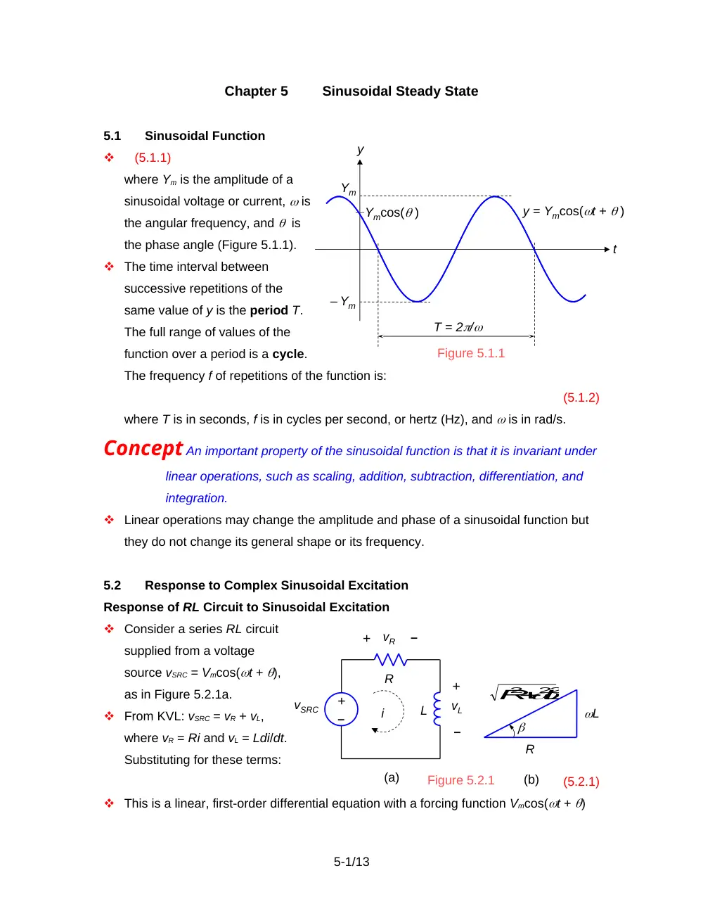
Chapter 5 Sinusoidal Steady State 5.1 Sinusoidal Function  (5.1.1) where Ym is the amplitude of a sinusoidal voltage or current,  is the angular frequency, and  is the phase angle (Figure 5.1.1).  The time interval between successive repetitions of the same value of y is the period T. The full range of values of the function over a period is a cycle. The frequency f of repetitions of the function is: (5.1.2) where T is in seconds, f is in cycles per second, or hertz (Hz), and  is in rad/s. Concept An important property of the sinusoidal function is that it is invariant under linear operations, such as scaling, addition, subtraction, differentiation, and integration.  Linear operations may change the amplitude and phase of a sinusoidal function but they do not change its general shape or its frequency. 5.2 Response to Complex Sinusoidal Excitation Response of RL Circuit to Sinusoidal Excitation  Consider a series RL circuit supplied from a voltage source vSRC = Vmcos(t + ), as in Figure 5.2.1a.  From KVL: vSRC = vR + vL, where vR = Ri and vL = Ldi/dt. Substituting for these terms: (5.2.1)  This is a linear, first-order differential equation with a forcing function Vmcos(t + ) 5-1/13 y Ym T = 2/ Ymcos( ) Figure 5.1.1 – Ym t y = Ymcos(t +  ) vSRC R L i L R (a) (b) Figure 5.2.1 2 2 2 L R   – + + + – – vR vL on the RHS. The complete solution is the sum of two components:  A transient component that is the solution to the equation , and which dies out with time. A steady state is assumed to prevail only after the transient component has become insignificant.  A steady-state component iSS that satisfies Equation 5.2.1. Since the linear operations on the LHS of Equation 5.2.1 affect the amplitude and phase of iSS without affecting the frequency. we may consider iSS to be of the form: (5.2.2) where Im and  are unknowns to be determined so as to satisfy Equation 5.2.1.  Substituting iSS from Equation 5.2.2 in Equation 5.2.1: (5.2.3)  If the LHS of Equation 5.2.3 is multiplied and divided by , it becomes: (5.2.4)  Let  be the angle whose sine is and whose cosine is therefore (Figure 5.2.1b). Equation 5.2.4 becomes: or: (5.2.5)  To equalize both sides of Equation 5.2.5 under all conditions, we must have and  = . It follows that: , (5.2.6) Response of RL Circuit to Complex Sinusoidal Excitation  Let: (5.2.7)  Since the circuit is linear, superposition applies, and iSS = iSS1 + iSS2, where iSS1 is the steady-state response to Vmcos(t + ), as given by Equation 5.2.6, and iSS2 is the steady-state response to jVmsin(t + ).  The excitation jVmsin(t + ) may be written as . Hence, iSS2 can be obtained from iss1 by replacing  by ( –) and multiplying Vm by j. This gives: , (5.2.8) 5-2/13 Concept When a complex sinusoidal excitation vSRC is applied to an LTI circuit, the response is a complex sinusoidal function whose real part is the response to the real part of the excitation, Vmcos(t + ), applied alone, and whose imaginary part is the response to the imaginary part of the excitation, Vmsin(t + ), applied alone.  In other words, the real and imaginary parts retain their separate identities in linear operations, without any mutual interaction. 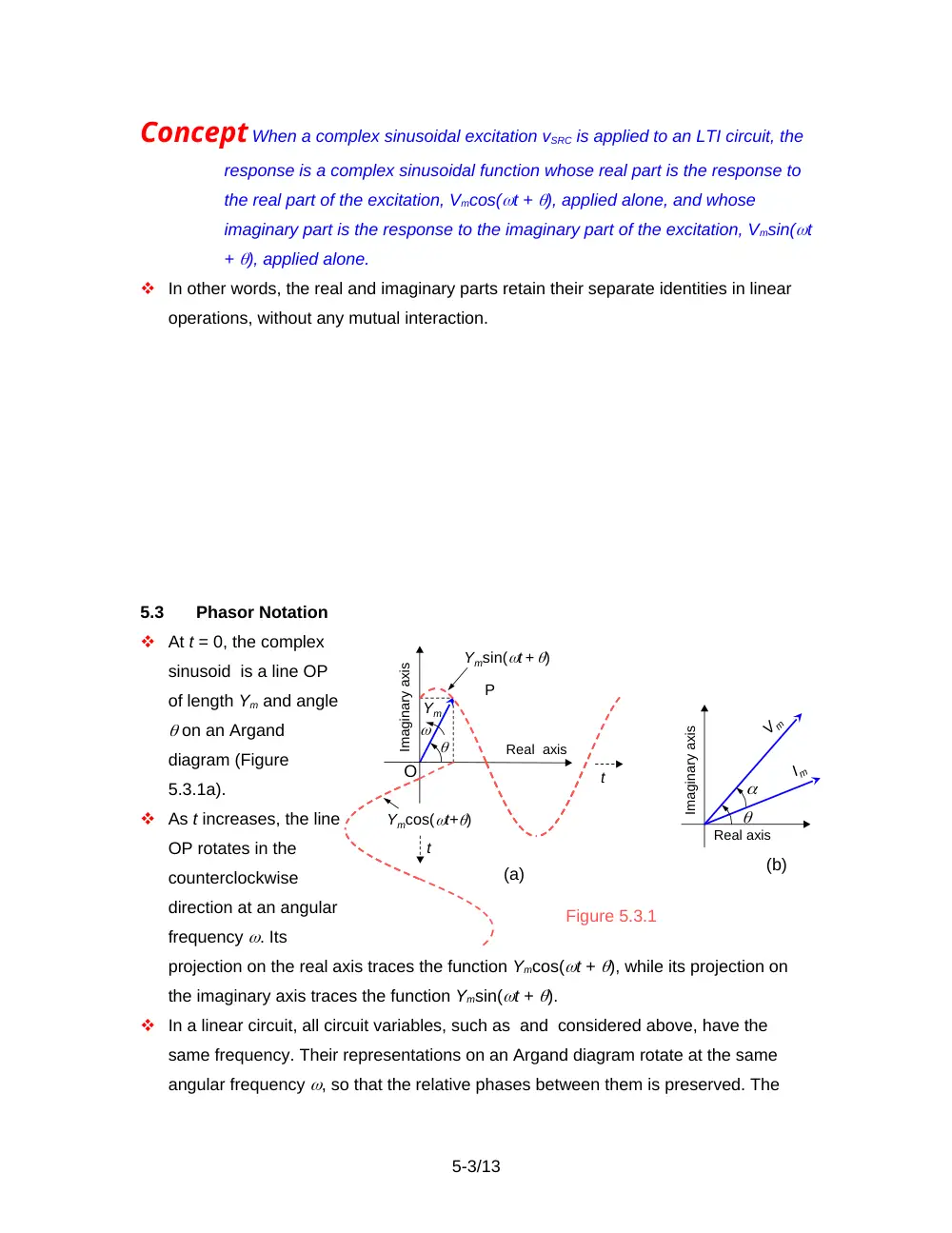5.3 Phasor Notation  At t = 0, the complex sinusoid is a line OP of length Ym and angle  on an Argand diagram (Figure 5.3.1a).  As t increases, the line OP rotates in the counterclockwise direction at an angular frequency . Its projection on the real axis traces the function Ymcos(t + ), while its projection on the imaginary axis traces the function Ymsin(t + ).  In a linear circuit, all circuit variables, such as and considered above, have the same frequency. Their representations on an Argand diagram rotate at the same angular frequency , so that the relative phases between them is preserved. The 5-3/13 Figure 5.3.1 Imaginary axis Real axis  Vm Im (a) (b) P Ym   t t Ymsin(t + )  Ymcos(t+) O Real axis Imaginary axis rotation can be frozen at t = 0 without loss of the information contained in the magnitudes and relative phase angles (Figure 5.3.1b). Definition A phasor is a quantity such as or representing a complex sinusoidal function of time, but with the time variation suppressed. Phasors are written in boldface and expressed as a magnitude and phase angle: V (5.3.1) Properties of Phasors  Since phasors have magnitude and direction, they are similar to vectors in many respects, but have a real part, Yr = Ymcos, and an imaginary part, Yi = Ymsin. It follows that .  Multiplying a phasor by a real quantity K multiplies its magnitude by K, without changing its phase angle. 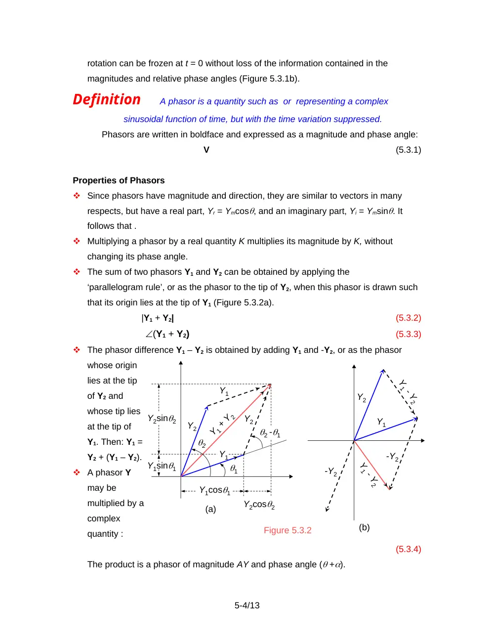 The sum of two phasors Y1 and Y2 can be obtained by applying the ‘parallelogram rule’, or as the phasor to the tip of Y2, when this phasor is drawn such that its origin lies at the tip of Y1 (Figure 5.3.2a). |Y1 + Y2| (5.3.2) (Y1 + Y2) (5.3.3)  The phasor difference Y1 – Y2 is obtained by adding Y1 and -Y2, or as the phasor whose origin lies at the tip of Y2 and whose tip lies at the tip of Y1. Then: Y1 = Y2 + (Y1 – Y2).  A phasor Y may be multiplied by a complex quantity : (5.3.4) The product is a phasor of magnitude AY and phase angle ( +). 5-4/13 Figure 5.3.2 (a) (b) 1 2 2 -1 Y1 Y1 Y2 Y2 Y1 + Y2 Y1cos1 Y2cos2 Y2sin2 Y1sin1 Y2 -Y2 Y1 -Y2 Y1 - Y2 Y1 - Y2  A phasor Y may be divided by a complex quantity : (5.3.5) The quotient is a phasor of magnitude and phase angle ( –).  In the complex plane, j is an imaginary quantity of unit magnitude and a phase angle of  /2: (5.3.6)  Multiplying a phasor by j rotates the phasor through an angle  /2 counterclockwise without changing its magnitude. Dividing a phasor by j, or conversely multiplying it by –j, since , rotates the phasor through an angle  /2 clockwise without changing its magnitude. Example 5.3.1 Magnitude, Real Part, and Imaginary Part of a Complex Fraction It is required to determine the magnitude, real, and imaginary parts of . Solution: Let us rationalize Y, i.e., make its denominator real, by multiplying numerator and denominator by the complex conjugate of the denominator, c – jd. Thus: (5.3.7) The real part of Y is its imaginary part is. The magnitude of Y may be obtained as the square root of the sum of the squares of the real and imaginary parts. An easier way is to convert the numerator and denominator to polar coordinates. Thus: . The magnitude of Y is therefore . It should be noted that, whereas the magnitude of Y is the magnitude of the numerator divided by that of the denominator, the real part of Y is not the real part of the numerator divided by that of the denominator. Nor is the imaginary part of Y the imaginary part of the numerator divided by that of the denominator. 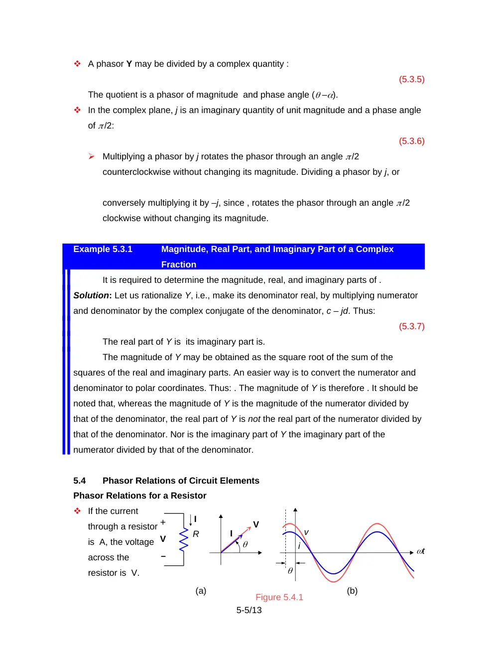5.4 Phasor Relations of Circuit Elements Phasor Relations for a Resistor  If the current through a resistor is A, the voltage across the resistor is V. 5-5/13 V + R I (a) i t v (b) Figure 5.4.1 V I   – In phasor notation (Figure 5.4.1a): VI, or IV (5.4.1)  According to the interpretation of complex sinusoidal excitation, a voltage Vmcos(t + ) V produces a current A that is in phase (Figure 5.4.1b).  The energy dissipated in a resistor R over a period is: (5.4.2)  The average power dissipated is: (5.4.3)  The operations leading to Equation 5.4.3 involve squaring the current Imcos(t + ), then taking the mean value over a period, which is . Similarly, the mean square of the voltage is . The square roots of these quantities are the root-mean-square (rms), values. Thus: , and (5.4.4)  The power dissipated may be expressed in terms of rms values as: W (5.4.5)  Since the power dissipated in R by a dc current I is W, it follows that: Concept A current of rms value Irms, or a voltage of rms value Vrms, dissipate the same power in a given resistor as a dc current, or a dc voltage, of the same value. Phasor Relations for an Inductor  If the inductor current is A, the inductor voltage is: V (5.4.6)  In phasor notation, I A, and V V, or: VI, or IV (5.4.7)  The magnitude of V is L times that of I, and the phase angle of V is  /2 plus the phase angle of I (Figure 5.4.2a). 5-6/13 jL (a) (b)  I V Im Vm V + I – Figure 5.4.2 i t v  Q P According to the interpretation of complex sinusoidal excitation, if the inductor current is: A, the inductor voltage is: V. The voltage leads the current by 90, or the current lags the voltage by 90 (Figure 5.4.2b). 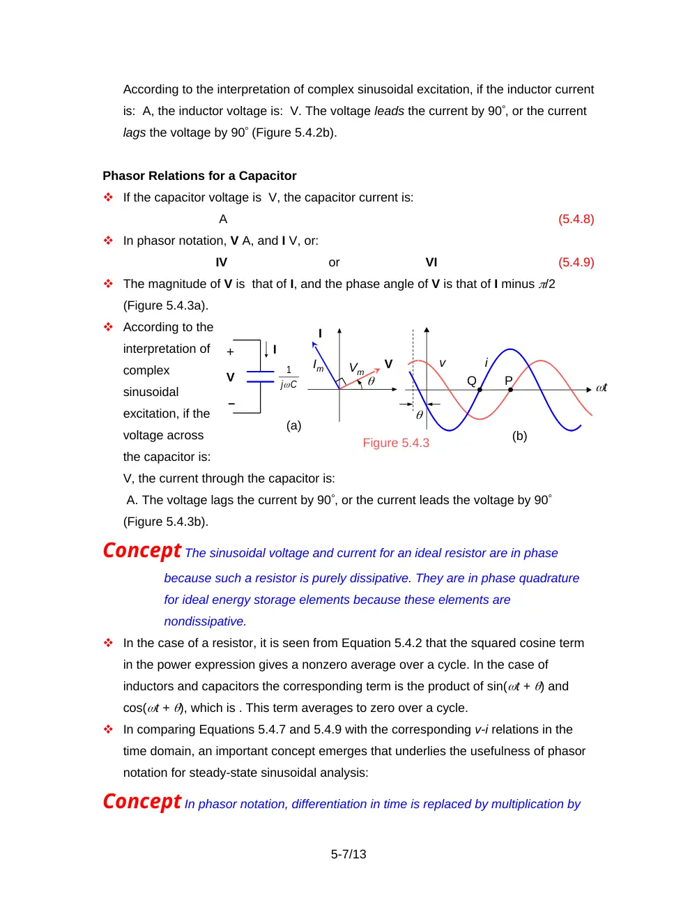Phasor Relations for a Capacitor  If the capacitor voltage is V, the capacitor current is: A (5.4.8)  In phasor notation, V A, and I V, or: IV or VI (5.4.9)  The magnitude of V is that of I, and the phase angle of V is that of I minus /2 (Figure 5.4.3a).  According to the interpretation of complex sinusoidal excitation, if the voltage across the capacitor is: V, the current through the capacitor is: A. The voltage lags the current by 90, or the current leads the voltage by 90 (Figure 5.4.3b). Concept The sinusoidal voltage and current for an ideal resistor are in phase because such a resistor is purely dissipative. They are in phase quadrature for ideal energy storage elements because these elements are nondissipative.  In the case of a resistor, it is seen from Equation 5.4.2 that the squared cosine term in the power expression gives a nonzero average over a cycle. In the case of inductors and capacitors the corresponding term is the product of sin(t + ) and cos(t + ), which is . This term averages to zero over a cycle.  In comparing Equations 5.4.7 and 5.4.9 with the corresponding v-i relations in the time domain, an important concept emerges that underlies the usefulness of phasor notation for steady-state sinusoidal analysis: Concept In phasor notation, differentiation in time is replaced by multiplication by 5-7/13 (a)  I V Vm Im C j 1 I V + – Figure 5.4.3 i t v  Q P (b) j, and integration in time is replaced by division by j. Thus, differential and integral relations are transformed to algebraic relations in j for steady-state sinusoidal analysis ONLY. 5.5 Impedance and Reactance  Let be a voltage phasor and be a related current phasor, representing, for example, the voltage and current between any two nodes in a circuit, and let . Then: Definition Impedance Z is the ratio of the voltage phasor to the related current phasor : = Z (5.5.1)  When V is in volts and I is in amperes Z is in ohms. 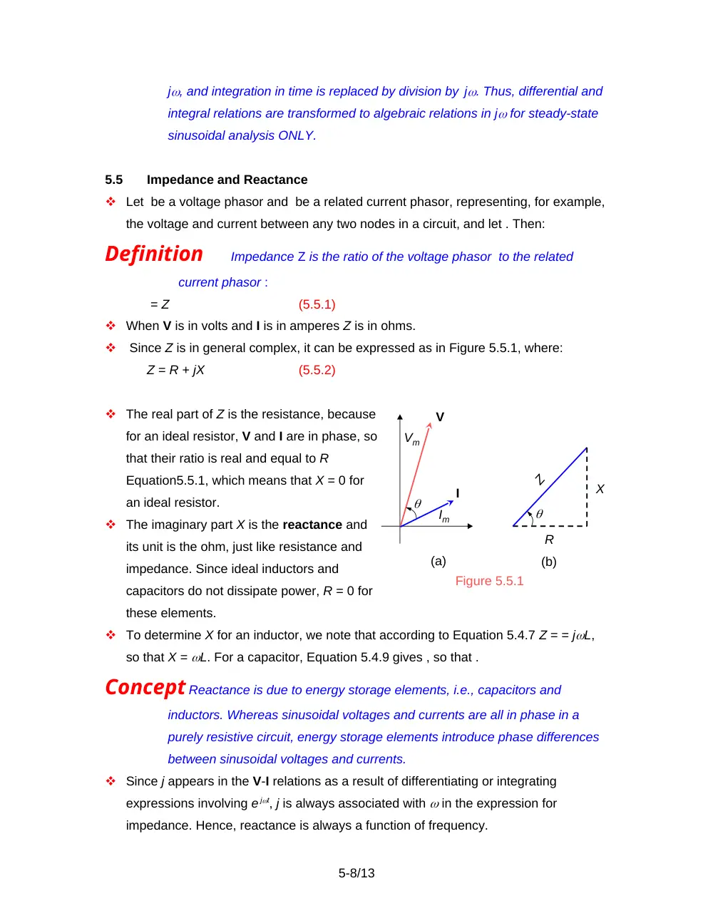 Since Z is in general complex, it can be expressed as in Figure 5.5.1, where: Z = R + jX (5.5.2)  The real part of Z is the resistance, because for an ideal resistor, V and I are in phase, so that their ratio is real and equal to R Equation5.5.1, which means that X = 0 for an ideal resistor.  The imaginary part X is the reactance and its unit is the ohm, just like resistance and impedance. Since ideal inductors and capacitors do not dissipate power, R = 0 for these elements.  To determine X for an inductor, we note that according to Equation 5.4.7 Z = = jL, so that X = L. For a capacitor, Equation 5.4.9 gives , so that . Concept Reactance is due to energy storage elements, i.e., capacitors and inductors. Whereas sinusoidal voltages and currents are all in phase in a purely resistive circuit, energy storage elements introduce phase differences between sinusoidal voltages and currents.  Since j appears in the V-I relations as a result of differentiating or integrating expressions involving e jt, j is always associated with  in the expression for impedance. Hence, reactance is always a function of frequency. 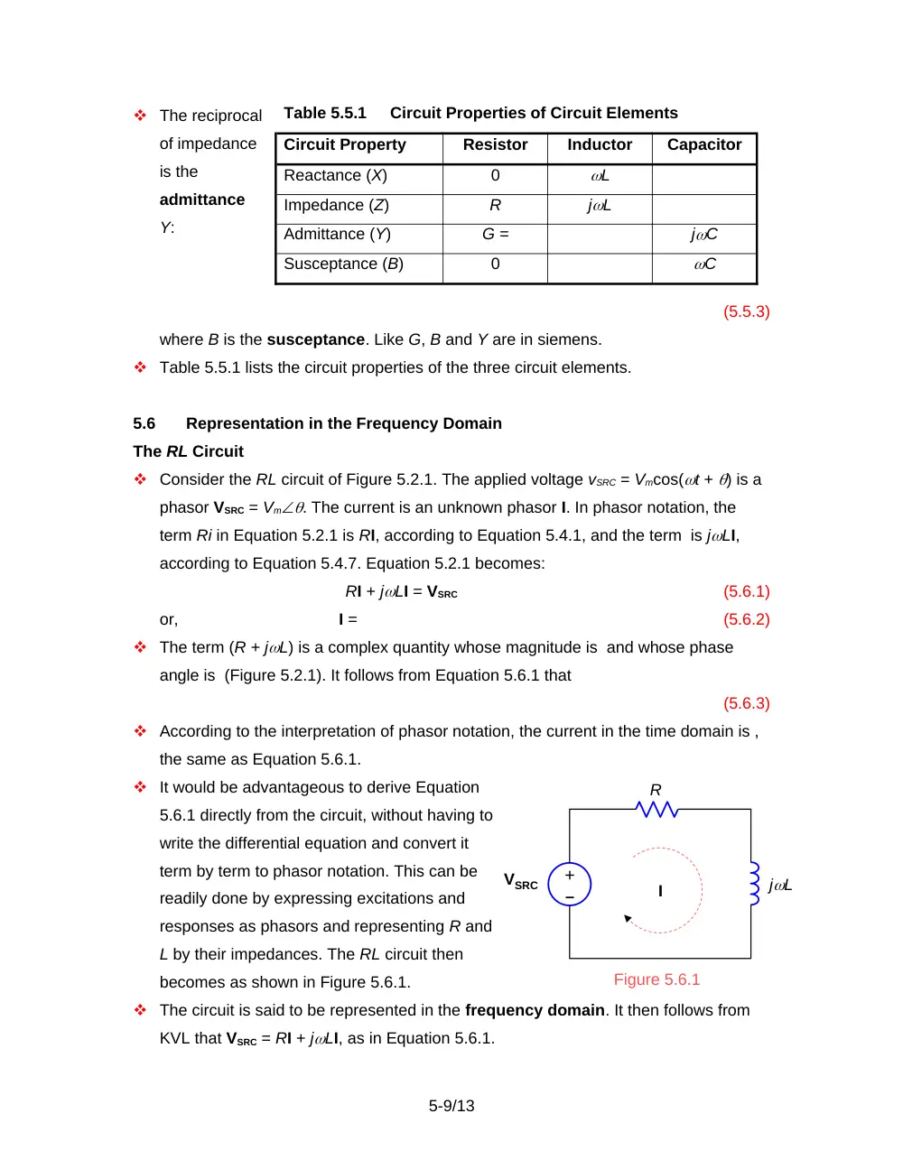5-8/13 V Z R X (a) (b) Figure 5.5.1  Im Vm  I  The reciprocal of impedance is the admittance Y: (5.5.3) where B is the susceptance. Like G, B and Y are in siemens.  Table 5.5.1 lists the circuit properties of the three circuit elements. 5.6 Representation in the Frequency Domain The RL Circuit  Consider the RL circuit of Figure 5.2.1. The applied voltage vSRC = Vmcos(t + ) is a phasor VSRC = Vm. The current is an unknown phasor I. In phasor notation, the term Ri in Equation 5.2.1 is RI, according to Equation 5.4.1, and the term is jLI, according to Equation 5.4.7. Equation 5.2.1 becomes: RI + jLI = VSRC (5.6.1) or, I = (5.6.2)  The term (R + jL) is a complex quantity whose magnitude is and whose phase angle is (Figure 5.2.1). It follows from Equation 5.6.1 that (5.6.3)  According to the interpretation of phasor notation, the current in the time domain is , the same as Equation 5.6.1.  It would be advantageous to derive Equation 5.6.1 directly from the circuit, without having to write the differential equation and convert it term by term to phasor notation. This can be readily done by expressing excitations and responses as phasors and representing R and L by their impedances. The RL circuit then becomes as shown in Figure 5.6.1.  The circuit is said to be represented in the frequency domain. It then follows from KVL that VSRC = RI + jLI, as in Equation 5.6.1. 5-9/13 Figure 5.6.1 + jL I R – VSRC Table 5.5.1 Circuit Properties of Circuit Elements Circuit Property Resistor Inductor Capacitor Reactance (X) 0 L Impedance (Z) R jL Admittance (Y) G = jC Susceptance (B) 0 C  Since KVL, KCL, and the v-i relations of circuit elements can all be expressed in the frequency domain, it follows that: Concept All circuit relations and theorems that apply to resistive circuits under dc conditions apply for sinusoidal steady-state analysis in the frequency domain to circuits that include resistance, inductance, and capacitance, with voltages and currents represented as phasors and impedances of circuit elements replacing resistance.  It should be emphasized that phasor analysis applies to the sinusoidal steady state only. 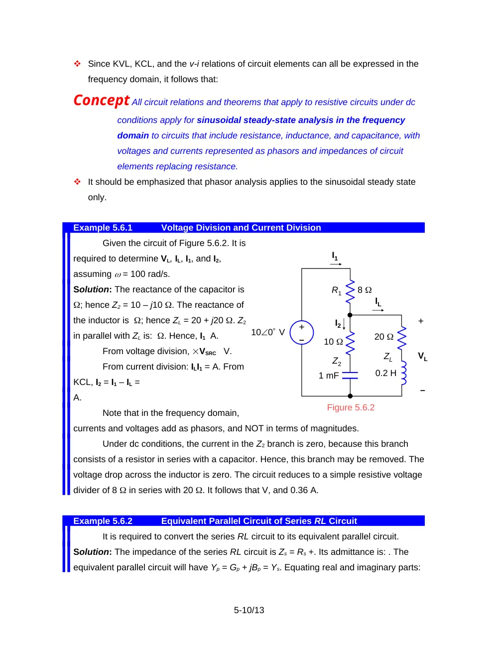Example 5.6.1 Voltage Division and Current Division Given the circuit of Figure 5.6.2. It is required to determine VL, IL, I1, and I2, assuming  = 100 rad/s. Solution: The reactance of the capacitor is ; hence Z2 = 10 – j10 . The reactance of the inductor is ; hence ZL = 20 + j20 . Z2 in parallel with ZL is: . Hence, I1 A. From voltage division, VSRC V. From current division: ILI1 = A. From KCL, I2 = I1 – IL = A. Note that in the frequency domain, currents and voltages add as phasors, and NOT in terms of magnitudes. Under dc conditions, the current in the Z2 branch is zero, because this branch consists of a resistor in series with a capacitor. Hence, this branch may be removed. The voltage drop across the inductor is zero. The circuit reduces to a simple resistive voltage divider of 8  in series with 20 . It follows that V, and 0.36 A. Example 5.6.2 Equivalent Parallel Circuit of Series RL Circuit It is required to convert the series RL circuit to its equivalent parallel circuit. Solution: The impedance of the series RL circuit is Zs = Rs +. Its admittance is: . The equivalent parallel circuit will have Yp = Gp + jBp = Ys. Equating real and imaginary parts: 5-10/13 I1 IL + VL Figure 5.6.2 + – – 100 V I2 8  10  20  1 mF 0.2 H R1 Z2 ZL , and (5.6.4) Both Gp and Bp are frequency dependent. At  = 0, Gp = and Bp = 0, as expected. For an ideal inductor, Rs = 0 = Gp and Bp = –1/Ls, also as expected. Gp can also be derived from the equality of power dissipation in Rs and Gp, since no power is dissipated in Ls or Bp, and the two circuits are equivalent at their respective terminals. The power dissipated in Rs is , whereas the power dissipated in Gp is . Equating these two quantities gives the same value of Gp. Example 5.6.3 Sinusoidal Steady State Using Node-Voltage Analysis It is required to analyze the circuit of Figure 5.6.4 by the node-voltage method, assuming  = 1 rad/s. The circuit configuration is the same as that of Figure 3.3.2. Solution: The admittance of the 20 H inductor is S, whereas that of the capacitor is j0.05 S. Following the usual procedure for writing the node- voltage equations, but using admittances instead of conductances, the node voltage equation for node e is: j0.05Vb – j0.05Vc – 0.1Vd +(0.1 – j0.05 + j0.05 + 0.1)Ve = 0. Substituting Vb = 10 gives: -j0.05Vc – 0.1Vd + 0.2Ve = -j0.5 For node c: -0.2Vb + (0.2 + j0.05)Vc – j0.05Ve = -I, and for node d: 0.1Vd – 0.1Ve = I + 0.1V. Adding these two equations to eliminate I and substituting Vb = 10 and V = Vc – Ve, gives: (0.1 + j0.05)Vc + 0.1Vd – j0.05Ve = 2 For the dependent voltage source, Vd – Vc = 2Vx = 2(Vb – Ve), or: -Vc + Vd + 2Ve = 20 Solving these three equations using MATLAB gives: Vc = 6.7568 – j0.5405 V, Vd = 13.2432 + j0.5405 V, and Ve = Vc = 6.7568 – j0.5405 V. Example 5.6.4 Sinusoidal Steady State Using Mesh-Current Analysis It is required to 5-11/13 + – – + I2 I Ix V1 I3 V2 20  2 H 40  20  5 mF + _ 100 V a 0.1V Vb b I 2Vx + + Vx V c d Vc Vd Ve – + – – e 10  5  10  50 mF Figure 5.6.4 20 H analyze the circuit of Figure 5.6.7 by the mesh-current method, assuming  = 10 rad/s. The circuit configuration is the same as that of Figure 3.5.2. Solution: The impedance of the 2 H inductor is j20 , that of the 5 mF capacitor is , and that of the 2 mF capacitor is –j50 . The mesh-current equation for mesh 1 is: 10I1 = -V1 – 4I, that for mesh 2 is: (60 + j20)I2 – 40I3 = V1. Adding and substituting I = I3: 10I1 + (60 + j20)I2 – 36I3 = 0 The mesh-current equation for mesh 3 is: (60 – j20)I3 – 40I2 = -V2, that for mesh 4 is: -j50I4 = V2 + 4I. Adding and substituting I = I3: -40I2 + (56 – j20)I3 – j50I4 = 0 For the independent current source: -I1 + I2 = 10 For the dependent current source: I4 – I3 = 2Ix, or: -2I2 – I3 + I4 = 0 Solving using MATLAB, gives: I1 = -8.9443 + j0.2038 A, I2 = 1.0557 + j0.2038 A, I3 = -0.8383 + j0.9828 A, and I4 = 1.2730 + j1.3904 A. 5.7 Phasor Diagrams  Phasor diagrams showing various voltage and current phasors in a given circuit are useful for illustrating the interrelations between the various variables involved, particularly when some circuit variable is varied. Example 5.7.1 Phase Shifter Given the circuit of Figure 5.7.1. It is required to determine how the output voltage vO changes as Rx is varied from 0 to infinity, assuming that no current is drawn at the output. Solution: The lattice configuration of Figure 5.7.1 may be redrawn as a bridge configuration, for easier visualization, and represented in the frequency domain as shown in Figure 5.7.2. 5-12/13 Rx R R C + vO vI = Vmcost + a b c d Figure 5.7.1 – – Since II, where , and the phasor I lags the phasor I by 90, then point Q joining these two phasors lies on the perimeter of a semicircle of diameter Vm (Figure 5.7.3). If a phasor I is drawn from point T at the tip of the phasor , then VOI is the phasor from the origin O to S at the tip of I. When Rx = 0, VO = and . Q coincides with O, and S coincides with T. As Rx increases, Q moves clockwise around the perimeter of its semicircle. Likewise, S moves clockwise around the perimeter of a semicircle because I is always parallel to I and of the same magnitude. As , I. Both plates of the capacitor will be at the same potential, and VO =. S would then lie at the tip of the phasor . At any Rx, VO = and . It is seen from the geometry that, where . Substituting, gives: . The circuit may be used to shift the phase of the output with respect to the input, without altering the magnitude. 5-13/13 Rx Rx 0 x R  x R c jX  O S Q T Rx I I Figure 5.7.3 VO – RxI Vm 0 Vm /20 – Vm /20 R R Rx RxI jXC I Vm/2 Vm/2 VO + + +  0  m V a b d c – – – – + + – Figure 5.7.2