EECE 491 Lecture 10, Spring 2016

Prof. M. Mansour EECE 491: Discrete-­‐time Signal Processing 1 EECE 491: Discrete-­‐time Signal Processing Mohammad M. Mansour Dept. of Electrical and Compute Engineering American University of Beirut Lecture 10: Sample-­‐Rate Conversion Prof. M. Mansour EECE 491: Discrete-­‐time Signal Processing 2 Announcements § Reading – O&S • Chapter 4 Prof. M. 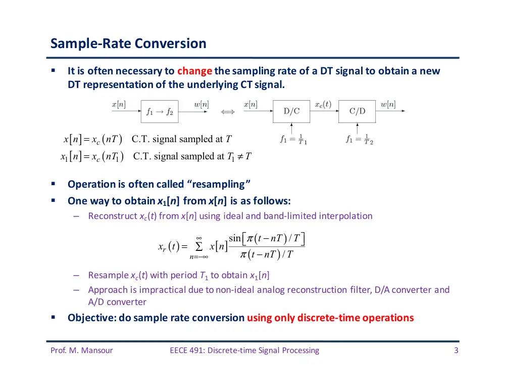Mansour EECE 491: Discrete-­‐time Signal Processing 3 Sample-­‐Rate Conversion § It is often necessary to change the sampling rate of a DT signal to obtain a new DT representation of the underlying CT signal. § Operation is often called “resampling” § One way to obtain x1[n] from x[n] is as follows: – Reconstruct xc(t) from x[n] using ideal and band-­‐limited interpolation – Resample xc(t) with period T1 to obtain x1[n] – Approach is impractical due to non-­‐ideal analog reconstruction filter, D/A converter and A/D converter § Objective: do sample rate conversion using only discrete-­‐time operations [ ] ( ) [ ] ( ) 1 1 1 C.T. signal sampled at C.T. signal sampled at c c x n x nT T x n x nT T T = = ≠ ( ) [ ] ( ) ( ) sin / / r n t nT T x t x n t nT T π π ∞ =−∞ − ⎡ ⎤ ⎣ ⎦ = ∑ − Prof. M. 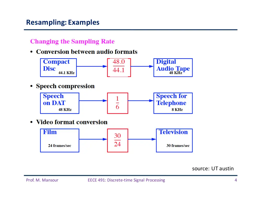Mansour EECE 491: Discrete-­‐time Signal Processing 4 Resampling: Examples source: UT austin Prof. M. Mansour EECE 491: Discrete-­‐time Signal Processing 5 Downsampling Prof. M. 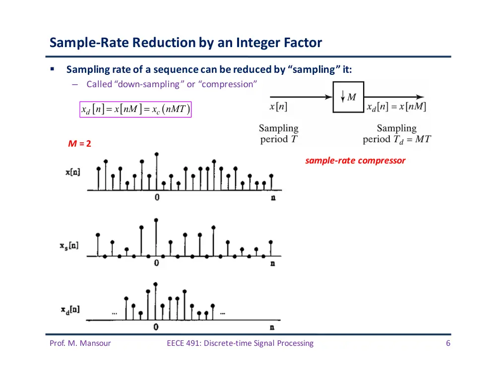Mansour EECE 491: Discrete-­‐time Signal Processing 6 Sample-­‐Rate Reduction by an Integer Factor § Sampling rate of a sequence can be reduced by “sampling” it: – Called “down-­‐sampling” or “compression” [ ] [ ] ( ) d c x n x nM x nMT = = sample-­‐rate compressor M = 2 Prof. M. 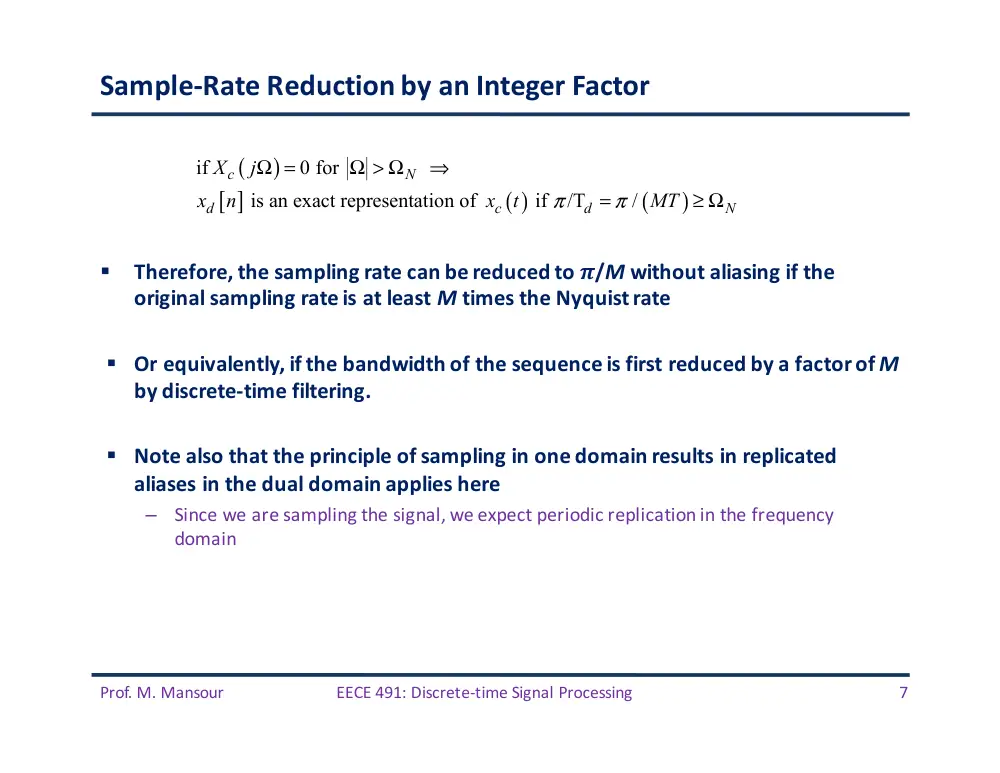Mansour EECE 491: Discrete-­‐time Signal Processing 7 Sample-­‐Rate Reduction by an Integer Factor § Therefore, the sampling rate can be reduced to 𝝅/M without aliasing if the original sampling rate is at least M times the Nyquist rate § Or equivalently, if the bandwidth of the sequence is first reduced by a factor of M by discrete-­‐time filtering. § Note also that the principle of sampling in one domain results in replicated aliases in the dual domain applies here – Since we are sampling the signal, we expect periodic replication in the frequency domain ( ) [ ] ( ) ( ) if 0 for is an exact representation of if /T / c N d c d N X j x n x t MT π π Ω = Ω > Ω ⇒ = ≥ Ω Prof. M. Mansour EECE 491: Discrete-­‐time Signal Processing 8 Frequency-­‐Domain Relationship of Downsampling [ ] ( ) ( ) 1 2 j c c k k x n x nT X e X j T T T ω ω π ∞ =−∞ ⎛ ⎞ ⎛ ⎞ = ⇒ = − ∑ ⎜ ⎟ ⎜ ⎟ ⎝ ⎠ ⎝ ⎠ [ ] [ ] ( ) ( ) 1 2 1 2 j d c d d c d r d d c r r x n x nM x nT X e X j T T T r X j MT MT MT ω ω π ω π ∞ =−∞ ∞ =−∞ ⎛ ⎞ ⎛ ⎞ = = ⇒ = − ∑ ⎜ ⎟ ⎜ ⎟ ⎝ ⎠ ⎝ ⎠ ⎛ ⎞ ⎛ ⎞ = − ∑ ⎜ ⎟ ⎜ ⎟ ⎝ ⎠ ⎝ ⎠ Set ; , 0 1 r i kM k i M = + − ∞ < < +∞ ≤ ≤ − ⇒ Xd e jω ( ) = 1 M 1 T Xc j ω MT − 2πk T − 2πi MT % &' ( )* % & ' ( ) * k=−∞ ∞ ∑ - . /0 1 2 30 =X e j ω−2πi ( )/ M % & ' ( ) * ! 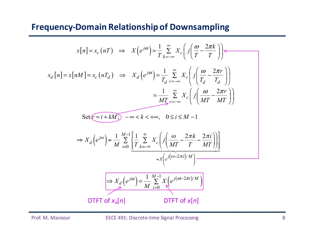" ###### $ ###### i=0 M−1 ∑ ( ) ( ) ( ) 1 2 / 0 1 M j i M j d i X e X e M ω π ω − − = ⇒ = ∑ DTFT of xd[n] DTFT of x[n] Prof. M. 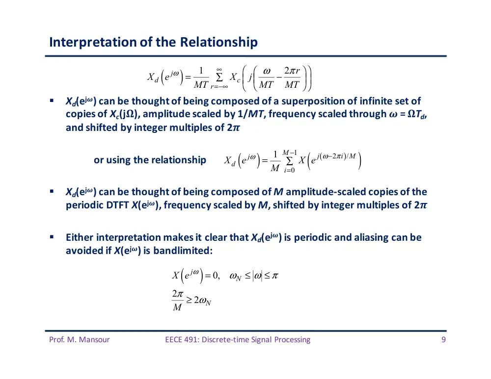Mansour EECE 491: Discrete-­‐time Signal Processing 9 Interpretation of the Relationship § Xd(ej𝝎) can be thought of being composed of a superposition of infinite set of copies of Xc(j𝛀), amplitude scaled by 1/MT, frequency scaled through 𝝎 = 𝛀Td, and shifted by integer multiples of 2𝝅 or using the relationship § Xd(ej𝝎) can be thought of being composed of M amplitude-­‐scaled copies of the periodic DTFT X(ej𝝎), frequency scaled by M, shifted by integer multiples of 2𝝅� § Either interpretation makes it clear that Xd(ej𝝎) is periodic and aliasing can be avoided if X(ej𝝎) is bandlimited: ( ) 1 2 j d c r r X e X j MT MT MT ω ω π ∞ =−∞ ⎛ ⎞ ⎛ ⎞ = − ∑ ⎜ ⎟ ⎜ ⎟ ⎝ ⎠ ⎝ ⎠ ( ) ( ) ( ) 1 2 / 0 1 M j i M j d i X e X e M ω π ω − − = = ∑ ( ) 0, 2 2 j N N X e M ω ω ω π π ω = ≤ ≤ ≥ Prof. M. 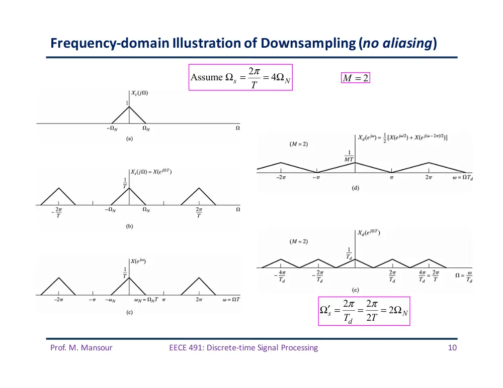Mansour EECE 491: Discrete-­‐time Signal Processing 10 Frequency-­‐domain Illustration of Downsampling (no aliasing) 2 Assume 4 s N T Ω = π = Ω 2 2 2 2 s N Td T π π ′ Ω = = = Ω M = 2 Prof. M. Mansour EECE 491: Discrete-­‐time Signal Processing 11 Frequency-­‐domain Illustration of Downsampling (with aliasing) 2 Assume 4 s N T Ω = π = Ω M = 3 2 N T π ⇒ Ω = 2 2 N NT T T π π ω = Ω = = 3 3 2 2 N N d T T T π π ω = Ω = = (aliasing occurs due to downsampling) In general aliasing occurs if 𝜔NM ≥ 𝜋 or 𝜔N ≥ 𝜋/M (to avoid aliasing, LPF X(ejΩ) with cutoff frequency 𝜔c = 𝜋/M before downsampling) Prof. M. Mansour EECE 491: Discrete-­‐time Signal Processing 12 Decimator § We saw that aliasing occurs due to downsampling if § To avoid aliasing, need to low-­‐pass filter x[n] with an ideal LPF with cutoff frequency 𝜔c = 𝜋/M before downsampling – The output can then be downsampled by a factor of M without aliasing § Downsampling by lowpass filtering followed by compression is called decimation – System is called decimator § Note: no longer represents the original underlying CT signal xc(t) – Rather, where Td = MT and is obtained from xc(t) by low-­‐pass filtering with cutoff frequency ωNM π ≥ !x n !" #$ !xd n !" #$= !x nM !" #$ !xd n !" #$= !xc nTd ( ) !xc t( ) ( ) / c Td MT π π Ω = = Sample-­‐rate compressor Downsampler or decimator DT filter Needed to avoid aliasing Prof. M. Mansour EECE 491: Discrete-­‐time Signal Processing 13 Upsampling Prof. M. Mansour EECE 491: Discrete-­‐time Signal Processing 14 Increasing the Sample-­‐Rate by an Integer Factor § Consider DT signal x[n] whose sample rate we wish to increase by a factor of L. – Underlying CT signal is xc(t) § Obtain § Increasing the sampling rate is called “upsampling” § We have [ ] ( ) [ ] ( ) , where / , from i c i i c x n x nT T T L x n x nT = = = Sample-­‐rate expander Upsampler or interpolator xi n[ ] = x n / L [ ] = x c nT / L ( ), when n = 0,±L,±2L,! DT filter Needed for interpolation Prof. M. Mansour EECE 491: Discrete-­‐time Signal Processing 15 (1) Expander: Time-­‐Domain Relations [ ] [ ] / 0, , 2 , 0 otherwise e x n L n L L x n = ± ± ⎧ = ⎨ ⎩ L Time domain illustration of expander with L = 2 [ ], 2 ex n L = [ ] [ ] [ ] or equivalently e k x n x k n kL δ ∞ =−∞ = − ∑ Prof. M. Mansour EECE 491: Discrete-­‐time Signal Processing 16 (2) Expander: Frequency-­‐Domain Relations [ ] [ ] [ ] e k x n x k n kL δ ∞ =−∞ = − ∑ ( ) [ ] [ ] [ ] ( ) j j n e n k j Lk k j L X e x k n kL e x k e X e ω ω ω ω δ ∞ ∞ − =−∞ =−∞ ∞ − =−∞ ⎛ ⎞ = − ∑ ⎜ ∑ ⎟ ⎝ ⎠ = ∑ = DTFT • Output DTFT is frequency-­‐ scaled version of DTFT of input • 𝝎 is replaced by 𝝎L 2 Assume 2 s N N T T π π Ω = = Ω ⇒ Ω = Prof. M. Mansour EECE 491: Discrete-­‐time Signal Processing 17 (3) Lowpass Filter § The LPF with gain L and cutoff frequency 𝝎c = 𝝅/L plays the role of the reconstruction filter to obtain xi[n] from xe[n] Assume N T π Ω = sampled at T sampled at / 2 iT T = reconstruction filter Prof. M. Mansour EECE 491: Discrete-­‐time Signal Processing 18 (3) Lowpass Filter § The reconstruction LPF, fills in the intermediate values to obtain xi[n] from xe[n] – Hence the reconstruction filter does interpolation [ ], 2 ex n L = [ ], ix n L = 2 Prof. M. Mansour EECE 491: Discrete-­‐time Signal Processing 19 Interpolation § Obtain a time-­‐domain relationship between xi[n] and x[n] § Impulse response of the LPF is § We have § hi[n] has the properties: – hi[0] = 1 – hi[n] = 0, for n = �L, �2L,… § Therefore, [ ] ( ) sin / ; cutoff / / i c n L h n L n L π ω π π = = [ ] [ ] [ ] [ ] [ ] [ ] i e e k x n x n h n x n x k n kL δ ∞ =−∞ = ∗ = − ∑ [ ] [ ] ( ) ( ) sin / / i k n kL L x n x k n kL L π π ∞ =−∞ − ⎡ ⎤ ⎣ ⎦ ⇒ = ∑ − [ ] [ ] ( ) ( ) / / , for all i c c i x n x n L x nT L x nT n = = = Prof. M. Mansour EECE 491: Discrete-­‐time Signal Processing 20 Practical Interpolators § Ideal LPFs for interpolation cannot be implemented exactly – PM algorithm gives good FIR approximations § Examine other forms of interpolation – Ex: linear interpolators Impulse  response  for  linear  interpolation. [ ] lin 1 / 0 otherwise n L n L h n − ≤ ⎧ = ⎨ ⎩ Prof. M. Mansour EECE 491: Discrete-­‐time Signal Processing 21 Example: Linear Interpolation by Filtering [ ] [ ] [ ] 1 lin lin 1 n L e k n L x n x k h n k + − = − + = − ∑ [ ] [ ] 0 0 ex = x [ ] [ ] 5 1 ex = x [ ] [ ] 10 2 ex x = [ ] [ ] 15 3 ex = x [ ] [ ] 20 4 ex = x [ ] [ ] 25 5 ex x = Original samples in xlin[n] are preserved since hi[0] = 1 and hi[n] = 0, for |n| ≥ L Prof. M. Mansour EECE 491: Discrete-­‐time Signal Processing 22 Example: Linear Interpolation by Filtering (cont’d) Nature of distortion in the intervening samples is better understood by comparing frequency responses of ideal and linear interpolators [ ] ( ) ( ) ( ) lin 2 1 / 0 otherwise sin / 2 1 sin / 2 j lin n L n L h n L H e L ω ω ω − ≤ ⎧ = ⎨ ⎩ ⎡ ⎤ = ⎢ ⎥ ⎣ ⎦ L = 5 If original sampling rate greatly exceeds Nyquist rate, signal will not vary significantly between samples, and hence linear interpolation will be more accurate for oversampled signals Prof. M. Mansour EECE 491: Discrete-­‐time Signal Processing 23 FIR Filters as Interpolators § Ideal bandlimited interpolators involve all original samples in the convolution of each interpolated sample § In contrast, linear interpolation involves only two § To get better approximation, use longer impulse responses § FIR filters are advantageous in this case. To interpolate by a factor L, they are usually designed with the following properties: !hi n !" #$ !hi n !" #$= 0, n ≥ KL !hi n !" #$= !hi −n !" #$, n ≤ KL !hi 0 !" #$=1, n = 0 !hi n !" #$= 0, n = ±L,±2L,",±KL !xi n !" #$= xe k !" #$ !hi n− k !" #$ k=n−KL+1 n+KL−1 ∑ Interpolated output Guarantee original signal samples are preserved in output !xi n !" #$= x n / L !" #$, at n = 0,±L,±2L," Filter will not introduce any phase shift into the interpolated samples Only 2K non-­‐zero samples within the region of support of are involved in the interpolation !hi n− k "# $% Prof. M. Mansour EECE 491: Discrete-­‐time Signal Processing 24 FIR Filters as Interpolators § Illustration of interpolation involving 2K = 4 samples when L = 5. – Each interpolated value depends on 2K = 4 samples of the original input – Computation requires only 2K multiplications and 2K – 1 additions since there are always L – 1 zero samples in xe[k] between each of the original samples § Higher-­‐order Lagrange interpolation formulas are possible from theory of numerical analysis Prof. M. Mansour EECE 491: Discrete-­‐time Signal Processing 25 Changing the Sample Rate by an Noninteger Factor § By combining decimation and interpolation, it is possible to change the sample rate by a noninteger factor Choosing L, M we get arbitrarily close to any desired ratio of sampling periods Prof. M. Mansour EECE 491: Discrete-­‐time Signal Processing 26 Example § Assume xc(t) is sampled at Nyquist rate 𝛀N=𝝅/T. § Want to change sampling Period to 3T/2. § Can choose L=2, M=3. § LPF has gain 2 and cutoff 𝝎c = min(𝝅/2, 𝝅/3)= 𝝅/3 Assume N T π Ω =