EECE 491 Lecture 6, Spring 2016

Prof. M. Mansour EECE 491: Discrete‐time Signal Processing 1 EECE 491: Discrete‐time Signal Processing Mohammad M. Mansour Dept. of Electrical and Compute Engineering American University of Beirut Lecture 6: Digital Filters Part I: Frequency Selective Filters Prof. M. Mansour EECE 491: Discrete‐time Signal Processing 2 Announcements  Reading – Chapter 5, Proakis Prof. M. Mansour EECE 491: Discrete‐time Signal Processing 3 Outline  Ideal Filter Characteristics  Lowpass Filters (LPF)  Highpass Filters (HPF)  Bandpass Filters (BPF)  Digital Resonators  Notch Filters  Comb Filters  All‐Pass Filters  Inverse Systems  Minimum Phase Systems Prof. M. 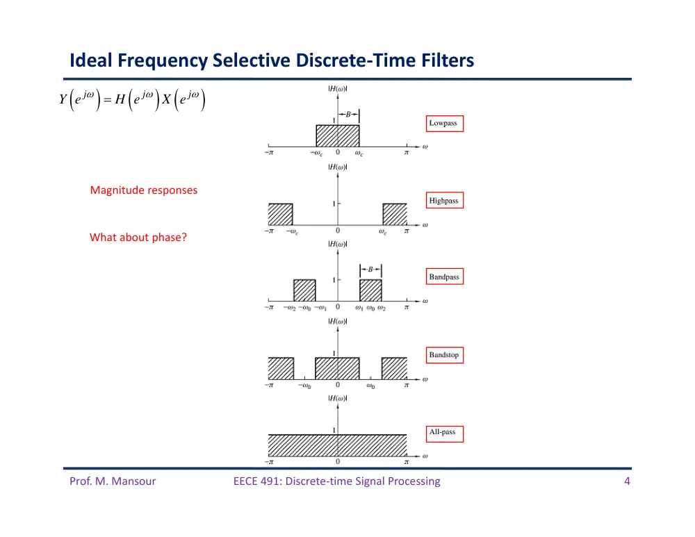Mansour EECE 491: Discrete‐time Signal Processing 4 Ideal Frequency Selective Discrete‐Time Filters Magnitude responses What about phase?       j j j Y e H e X e     Prof. M. 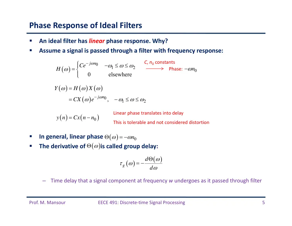Mansour EECE 491: Discrete‐time Signal Processing 5 Phase Response of Ideal Filters  An ideal filter has linear phase response. Why?  Assume a signal is passed through a filter with frequency response:  In general, linear phase  The derivative of          is called group delay: – Time delay that a signal component at frequency w undergoes as it passed through filter   0 1 2 0 elsewhere Ce j n H               C, n0 constants         0 1 2 j n , Y H X CX e                  0  y n Cx n n   Linear phase translates into delay This is tolerable and not considered distortion Phase:     g d d        n0    n0          Prof. M. 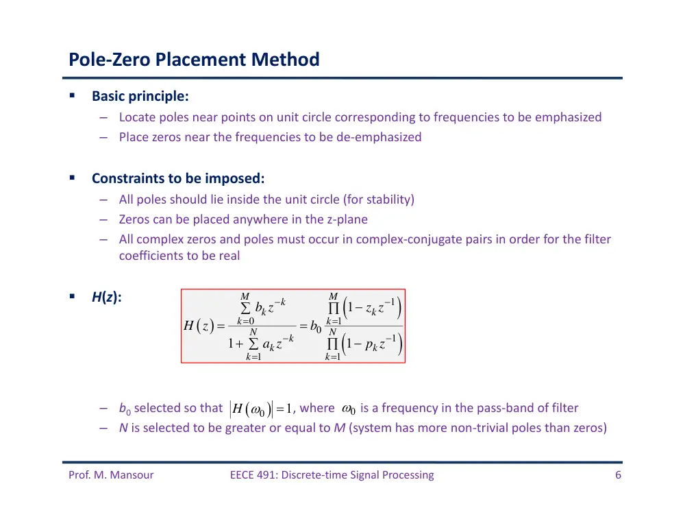Mansour EECE 491: Discrete‐time Signal Processing 6 Pole‐Zero Placement Method  Basic principle: – Locate poles near points on unit circle corresponding to frequencies to be emphasized – Place zeros near the frequencies to be de‐emphasized  Constraints to be imposed: – All poles should lie inside the unit circle (for stability) – Zeros can be placed anywhere in the z‐plane – All complex zeros and poles must occur in complex‐conjugate pairs in order for the filter coefficients to be real  H(z): – b0 selected so that , where is a frequency in the pass‐band of filter – N is selected to be greater or equal to M (system has more non‐trivial poles than zeros)       1 0 1 0 1 1 1 1 1 1 M M k k k k k N N k k k k k z z b z H z b a z p z                   0  1 H   0 Prof. M. 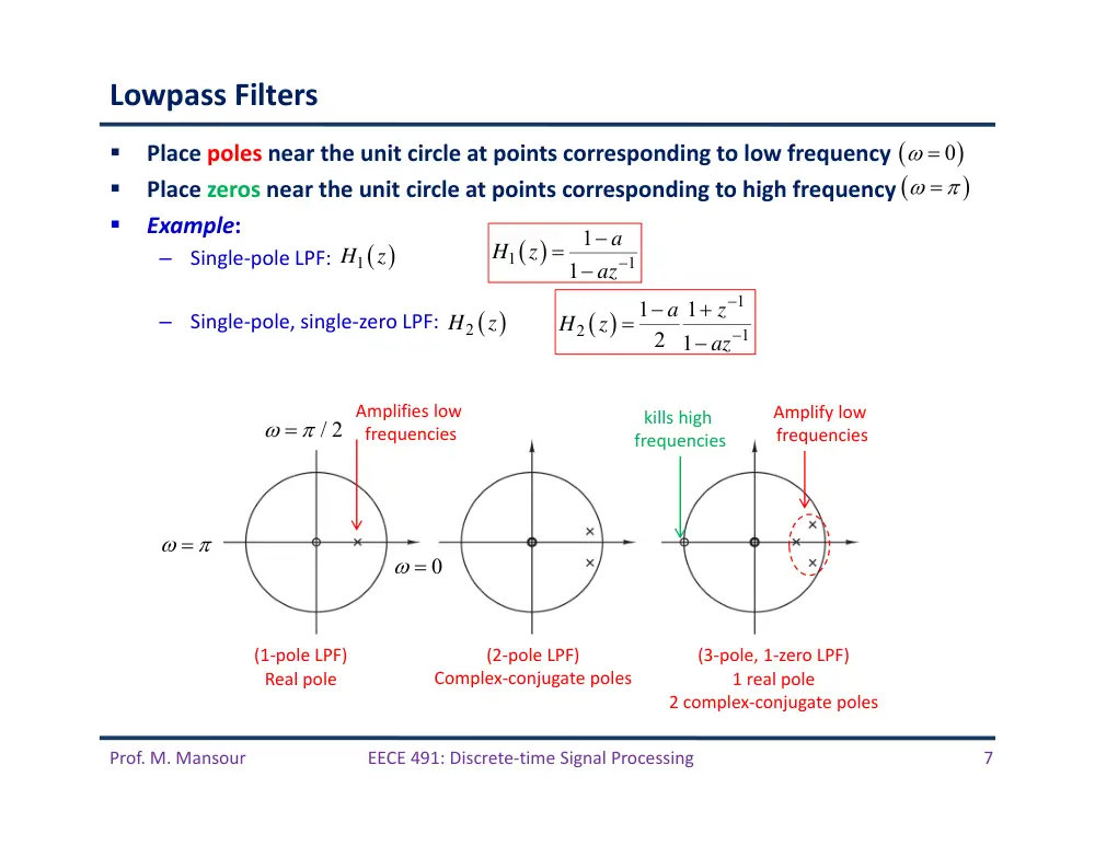Mansour EECE 491: Discrete‐time Signal Processing 7 Lowpass Filters  Place poles near the unit circle at points corresponding to low frequency  Place zeros near the unit circle at points corresponding to high frequency  Example: – Single‐pole LPF: – Single‐pole, single‐zero LPF: 1   1 1 1 a H z az      1 2 1 1 1 2 1 a z H z az       (2‐pole LPF) Complex‐conjugate poles (1‐pole LPF) Real pole (3‐pole, 1‐zero LPF) 1 real pole 2 complex‐conjugate poles Amplifies low frequencies kills high frequencies Amplify low frequencies  0        H1   z H2   z / 2         0 Prof. M. 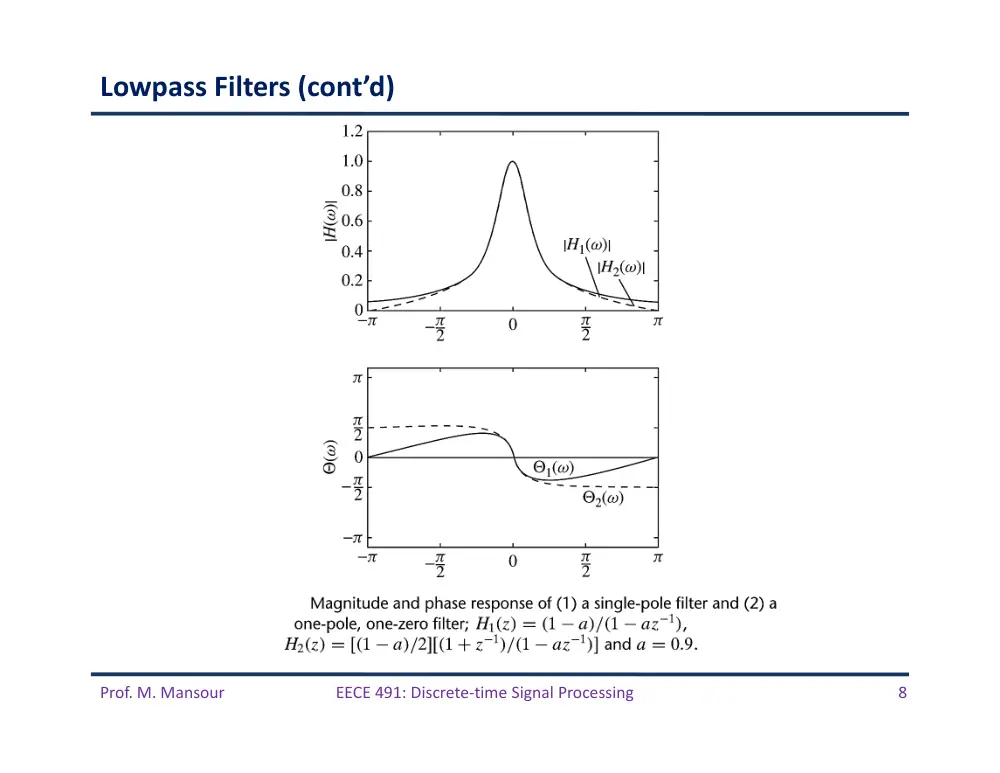Mansour EECE 491: Discrete‐time Signal Processing 8 Lowpass Filters (cont’d) Prof. M. 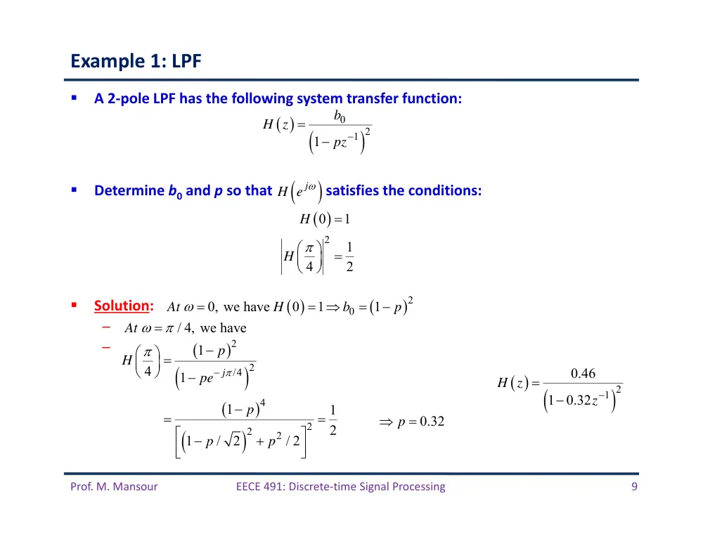Mansour EECE 491: Discrete‐time Signal Processing 9 Example 1: LPF  A 2‐pole LPF has the following system transfer function:  Determine b0 and p so that satisfies the conditions:  Solution: – . –     0 1 2 1 b H z pz     2 0 1 1 4 2 H H          0.32  p      1 2 0.46 1 0.32 H z z     j H e      2 0 0, we have 0 1 1 At H b p       / 4, we have At            2 2 /4 4 2 2 2 1 4 1 1 1 2 1 / 2 / 2 j p H pe p p p                        Prof. M. Mansour EECE 491: Discrete‐time Signal Processing 10 Highpass Filters  Pole‐zero placement  Simply reflect the pole‐zero locations of the low‐pass filters about the imaginary axis  Same ideas can be extended to design bandpass filters   1 3 1 1 1 2 1 a z H z az       Prof. M. Mansour EECE 491: Discrete‐time Signal Processing 11 Highpass Filters (cont’d) Prof. M. Mansour EECE 491: Discrete‐time Signal Processing 12 Example 2: BPF  Design a 2‐pole bandpass filter that has the center of its bandpass at                   , zero in its frequency response characteristic at             and               , and a magnitude of              at  Solution: The filter must have: – Poles at – Zeros at  Hence, system function looks like:  Gain factor G is chosen such that H has unit gain at center frequency:  Parameter r determined from :         BPF 2 2 2 1 1 1 z z H z G z jr z jr G z z r         2 2 2 1 1 2 2 1 r H G G r                    2 2 2 2 4 2 1 2 2cos 8 / 9 4 1 0.7 9 2 4 1 2 cos 8 / 9 r H r r r                    2 BPF 2 0.15 1 1 0.7 z H z z      / 2      0    1/ 2 4 / 9    /2 1,2 j p re jr      1 1 and 2 1 z z       at 4 / 9 H     Prof. M. Mansour EECE 491: Discrete‐time Signal Processing 13 Example 2: BPF (cont’d) Prof. M. Mansour EECE 491: Discrete‐time Signal Processing 14 A Lowpass to Highpass Filter Transformation  Given a Lowpass filter             with frequency response  A Highpass filter can be obtained by translating                  by      radians:  In time domain, this corresponds to multiplication by – Change the signs of the odd‐numbered samples of  LPF:  HPF:     HP LP j j H e H e                HP LP LP 1 n n j h n e h n h n           1 0 N M k k k k y n a y n k b x n k            0 LP 1 1 M j k k j k N j k k k b e H e a e                  0 HP 1 1 1 1 M k j k k j k N k j k k k b e H e a e                             1 0 1 1 N M k k k k k k y n a y n k b x n k            hLP   n   j HLP e    j HLP e   j n e  hLP   n Prof. M. Mansour EECE 491: Discrete‐time Signal Processing 15 Digital Resonators  A Special 2‐pole bandpass filter with the pair of complex‐conjugate poles located near the unit circle  Resonator: Filter “resonates” in the vicinity of the pole location  Applications: Bandpass filtering and speech recognition Prof. M. Mansour EECE 491: Discrete‐time Signal Processing 16 Digital Resonators  For a resonant peak frequency at or near : – Select the complex conjugate poles to be  We can select up to two zeros: – Choice 1 H1(z): select both zeros to be at origin – Choice 2 H2(z): select zeros to be at z = +1 and z = –1. This choice eliminates frequencies � � 0 and � � � which is useful in many applications  For choice 1, we have  Gain at �0 is 1:              0 1 1 1 0 0 0 1 0 0 0 0 0 0 2 0 1 1 1 1 1 1 j j j j j j j b H z re z re z b H re e re e b r re                               0 1 0 2 0 2 0 0 1 1 1 2 cos2 1 1 2 cos2 b H r r r b r r r              0    0 1,2 , 0 1 j p re r        0 Prof. M. Mansour EECE 491: Discrete‐time Signal Processing 17 Digital Resonators  At frequency �, we have        2 0 1 0 0 1 1 2 cos2 1 1 j j j j r r r H re e re e                        2 0 1 1 2 1 1 2 cos2 r r r H U U               1 2 2           �� x x � ��� � �� (�) �� (�)         2 1 0 2 2 0 1 2 cos 1 2 cos U r r U r r                   1 2 U  U  reaches its minimum at frequency 2 1 0 1 cos cos 2 r r r              (resonant frequency) As r → 1, �� → �0 Prof. M. Mansour EECE 491: Discrete‐time Signal Processing 18 Digital Resonators  As � approaches 1, the resonant peak becomes sharper  A quantitative measure is the 3dB bandwidth ∆�: – For � close to 1, ∆� ≈ 2(1−�) Prof. M. Mansour EECE 491: Discrete‐time Signal Processing 19 Digital Resonators (cont’d)  Choice 2: select zeros to be at � = +1 and � = −1                   1 1 2 1 1 0 0 2 2 0 0 1 1 1 1 1 1 1 j j j j j z z H z G re z re z e H G re re                           Prof. M. Mansour EECE 491: Discrete‐time Signal Processing 20 Notch Filters  Contains perfect nulls in its frequency response characteristic – Used in applications where specific frequencies must be eliminated (e.g. power‐line 60 Hz and its harmonics in instrumentation systems)  FIR systems – To create a null at frequency ��, we introduce a pair of complex‐conjugate zeros on the unit circle at an angle ��        1 1 0 0 0 1 2 0 0 1 1 1 2cos j j H z b e z e z b z z               Nulls at �� and �� Prof. M. Mansour EECE 491: Discrete‐time Signal Processing 21 Notch Filters Nearby frequencies attenuated Prof. M. Mansour EECE 491: Discrete‐time Signal Processing 22 Notch Filters  Disadvantages of FIR notch filters – Frequencies components around the desired nulls are severely attenuated (i.e., the notch has a relatively large bandwidth)  Solution: Use IIR approach and introduce poles to amplify nearby frequencies  Place a pair of complex‐conjugate poles at – Effect: They introduce a resonance in the vicinity of the null and thus reduce the bandwidth of the notch (note the poles are not on the unit circle: 0 < � < 1)  System function: 0 1,2 j p re      1 2 0 0 1 2 2 0 1 2cos 1 2 cos z z H z b r z r z            Prof. M. Mansour EECE 491: Discrete‐time Signal Processing 23 Notch Filters Prof. M. Mansour EECE 491: Discrete‐time Signal Processing 24 Comb Filters  A notch filter in which the nulls occur periodically across the frequency band  Example: Moving average FIR  Has � zeros on the unit circle at:   2 / 1 , 1,2, , j k M k M z e          1 1 1 1 1 1 M z H z M z          /2 1 sin 2 1 sin / 2 j M j M e H e M                   0 1 1 M k y n x n k M      � = �� Prof. M. Mansour EECE 491: Discrete‐time Signal Processing 25 Comb Filters  In general, a comb filter can be created by taking an FIR filter with and replacing � by ��  ��(ej�) is an �‐order repetition of �(ej�) in the range � ≤ � ≤ �  If �(�) has a spectral null at some frequency ��, then ��(�) has periodically spaced nulls at �� = ��+ ���/� for �=�,�,…,�−�     0 M k k H z h k z        0 M kL L k H z h k z          0 M j jkL L k jL H e h k e H e         Prof. M. Mansour EECE 491: Discrete‐time Signal Processing 26 Comb Filters Prof. M. Mansour EECE 491: Discrete‐time Signal Processing 27 Comb Filters Prof. M. Mansour EECE 491: Discrete‐time Signal Processing 28 Comb Filters  Back to moving average FIR  Has zeros at – For all integer values of � except � = 0, �, 2�, …     1 1 1 1 1 1 M z H z M z        � → ��    1 1 1 1 1 L M L L z H z M z          /2 1 sin 1 2 1 sin / 2 j LM L L M H e M L                 2 / 1 j k L M z e    Prof. M. Mansour EECE 491: Discrete‐time Signal Processing 29 All‐Pass Filters  Has constant response for all frequencies, but phase varies  Used to alter phase characteristics of a system, e.g., equalization  Simplest all pass system is delay system  Another system:  Since – Then the system is all‐pass system  If �� is a pole of �(�) then �/�� is a zero of �(�). Poles and zeros are reciprocals of one another   1, 0 j H e         k H z z        2 1 1 z e j H H z H z       Prof. M. Mansour EECE 491: Discrete‐time Signal Processing 30 All‐Pass Filters Prof. M. Mansour EECE 491: Discrete‐time Signal Processing 31 All‐Pass Filters  General form of all‐pass filters (real coefficients)         1 1 * 1 ap 1 1 * 1 1 1 1 1 1 N N C R k k k k k k k k z z z H z z z z                        Prof. M. Mansour EECE 491: Discrete‐time Signal Processing 32 Inverse Systems                     * * * 1 I I I w n h n h n x n x n h n h n n H z H z      Prof. M. Mansour EECE 491: Discrete‐time Signal Processing 33 Minimum‐Phase Systems  Invertibility of an LTI system is related to the characteristics of the phase spectral function of the system  Example:  In frequency domain:     1 1 1 1 1 2 1 1 1 2 2 1 1 1 2 2 H z z z z H z z z z                             1 2 5 cos 4 H H       1   sin arctan 1 cos 2          2   sin arctan 2 cos          Net phase change is 0  Minimum phase system Net phase change is  Maximum phase system Has zero inside unit circle Has zero outside unit circle Prof. M. Mansour EECE 491: Discrete‐time Signal Processing 34 Minimum‐Phase Systems  A minimum‐phase FIR system of length M + 1:  If all zeros are inside the unit circle, then each factor contributes a zero phase change, hence the overall system is minimum phase – Since group delay is derivative of phase, a minimum phase system has least delay  If all zeros are outside unit circle, then system is maximum phase  Otherwise it is called mixed‐phase system  Minimum‐phase IIR systems (stable and causal): – All poles and zeros are inside unit circle  Minimum phase property ensures that a stable system that is minimum phase has stable inverse which is also minimum phase