EECE 491 Lecture 7, Spring 2016

Prof. M. Mansour EECE 491: Discrete‐time Signal Processing 1 EECE 491: Discrete‐time Signal Processing Mohammad M. Mansour Dept. of Electrical and Compute Engineering American University of Beirut Lecture 7: Digital Filters Part II: FIR Filter Design Prof. M. Mansour EECE 491: Discrete‐time Signal Processing 2 Announcements  Reading – Chapter 10, Proakis – Chapter 7, O&S Prof. M. Mansour EECE 491: Discrete‐time Signal Processing 3 Outline  Causality and Implications  Characteristics of practical filters  Linear‐phase FIR filter types  Design of linear‐phase FIR filters using Windowing technique  Design of optimum equiripple linear‐phase FIR Filters – Alternation theorem – Parks‐McClellan algorithm Prof. M. 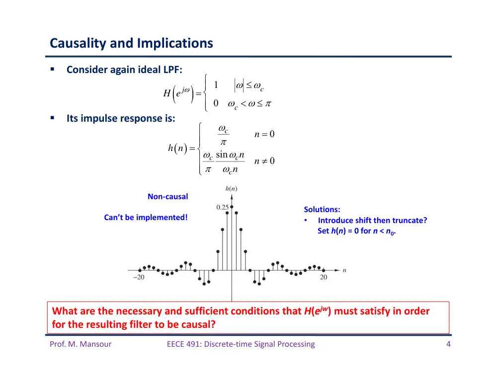Mansour EECE 491: Discrete‐time Signal Processing 4 Causality and Implications  Consider again ideal LPF:  Its impulse response is: H e j    1  c 0 c         0 sin 0 c c c c n h n n n n               Non‐causal Can’t be implemented! Solutions: • Introduce shift then truncate? Set h(n) = 0 for n < n0. What are the necessary and sufficient conditions that H(ejw) must satisfy in order for the resulting filter to be causal? Prof. M. Mansour EECE 491: Discrete‐time Signal Processing 5 Paley‐Wiener Theorem  Theorem: If h(n) has finite energy and h(n) = 0 for n < 0, then  Conversely, if H(ejw) is square‐integrable and if the above integral is finite, then we can associate with               a phase response           so that the resulting filter with response is causal.  Implications: – can be zero at some frequencies but not over a finite band of frequencies – Hence, any ideal filter (containing flat regions) is not causal  Causality imposes tight constraints on an LTI system  Causality also implies a strong relationship between – Real                 and imaginary components of – Magnitude                and phase of – Both pairs of quantities cannot be specified independently for a causal filter ln H e j   d      H e j    H e j   e j    H e j       H e j   HR e j   HI e j   H e j   H e j    e j   H e j   Prof. M. 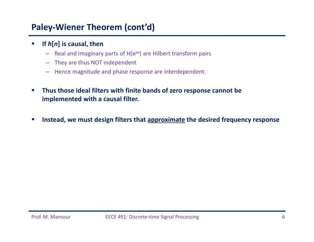Mansour EECE 491: Discrete‐time Signal Processing 6 Paley‐Wiener Theorem (cont’d)  If h[n] is causal, then – Real and Imaginary parts of H(ejw) are Hilbert transform pairs – They are thus NOT independent – Hence magnitude and phase response are interdependent.  Thus those ideal filters with finite bands of zero response cannot be implemented with a causal filter.  Instead, we must design filters that approximate the desired frequency response Prof. M. 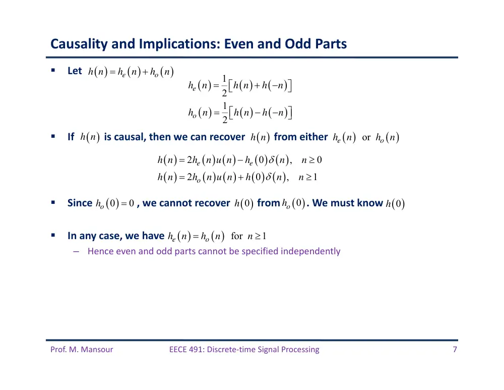Mansour EECE 491: Discrete‐time Signal Processing 7 Causality and Implications: Even and Odd Parts  Let  If is causal, then we can recover from either  Since                 , we cannot recover from          . We must know  In any case, we have – Hence even and odd parts cannot be specified independently       e o h n h n h n               1 2 1 2 e o h n h n h n h n h n h n                                   2 0 , 0 2 0 , 1 e e o h n h n u n h n n h n h n u n h n n           h n   h n     or e o h n h n   0 0 ho    h 0   ho 0   0 h     for 1 e o h n h n n   Prof. M. 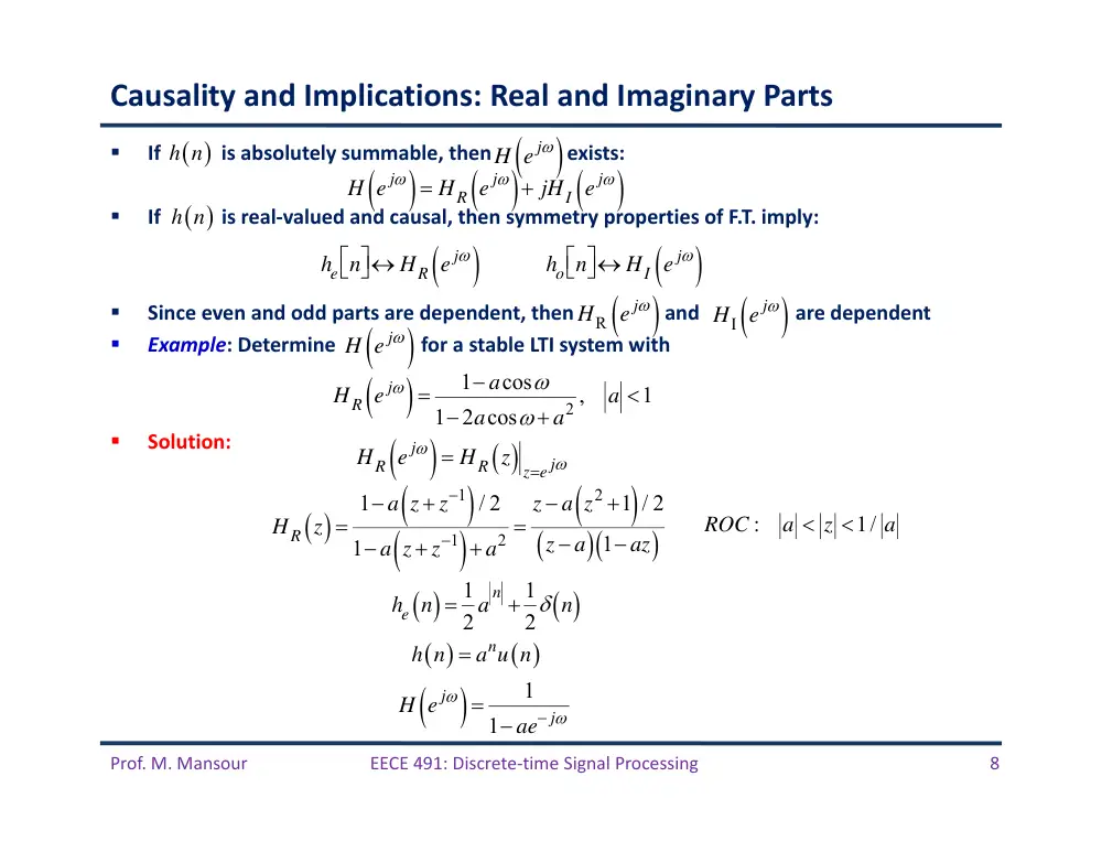Mansour EECE 491: Discrete‐time Signal Processing 8 Causality and Implications: Real and Imaginary Parts  If            is absolutely summable, then               exists:  If is real‐valued and causal, then symmetry properties of F.T. imply:  Since even and odd parts are dependent, then                  and                   are dependent  Example: Determine                 for a stable LTI system with  Solution: H e j    HR e j   jHI e j   he n   HR e j   ho n   HI e j   HR e j    1 acos 12acos  a2 , a 1 HR e j    HR z  ze j HR z   1 a z  z1   / 2 1 a z  z1   a2  z  a z2 1   / 2 z  a  1 az   : 1/ ROC a z a   he n   1 2 a n  1 2 n    n   h n a u n  H e j    1 1 ae j   h n   h n H e j   HI e j   HR e j   H e j   Prof. M. Mansour EECE 491: Discrete‐time Signal Processing 9 Solution (cont’d) z  a z2 1   / 2 z  a  1 az    az2  2z  a 2 az2  a2 1   z  a    az2  2z  a a2 1   z  a2 1   z 2 az2  a2 1   z  a    1 2  1 a2  z 2 z  a   1 az    1 2  a / 2 z  a  1/ 2 1 az  1 2  1/ 2 1 z / a  1/ 2 1 az he n   1 2 n   1 2 1 a     n u n1   1 2 anu n    1 2 n   1 2 anu n1   1 2 anu n    1 2 n   1 2 a n a 1 ROC : a  z 1/ a      1 n n x n u n b u n        1 1 1 1 1 1 X z z bz          ROC z : z b     Prof. M. 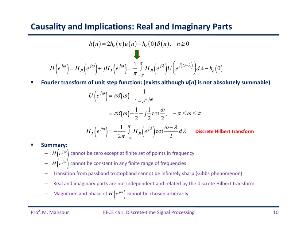Mansour EECE 491: Discrete‐time Signal Processing 10 Causality and Implications: Real and Imaginary Parts  Fourier transform of unit step function: (exists although u[n] is not absolutely summable)  Summary: – cannot be zero except at finite set of points in frequency – cannot be constant in any finite range of frequencies – Transition from passband to stopband cannot be infinitely sharp (Gibbs phenomenon) – Real and imaginary parts are not independent and related by the discrete Hilbert transform – Magnitude and phase of cannot be chosen arbitrarily           2 0 , 0 e e h n h n u n h n n     H e j    HR e j   jHI e j    1  HR e j  U e j       d  he 0     U e j        1 1 e j      1 2  j 1 2cot 2 ,     HI e j     1 2 HR e j  cot   2 d    Discrete Hilbert transform H e j   H e j   H e j   Prof. M. Mansour EECE 491: Discrete‐time Signal Processing 11 Characteristics of Practical Frequency‐Selective Filters Prof. M. Mansour EECE 491: Discrete‐time Signal Processing 12 Linear‐Phase FIR Filter Types Prof. M. Mansour EECE 491: Discrete‐time Signal Processing 13 Design of FIR Filters       1 0 M k y n h k x n k          1 0 M k k H z h k z                      2 1 1 2 0 1 2 2 1 M M H z h h z h z h M z h M z                                        3 /2 1 /2 1 2 /2 1 2 /2 0 /2 1 1 /2 1 2 /2 1 2 /2 0 1 , odd 2 , even M M M k M k n M M M k M k n M z h h n z z M H z z h n z z M                                                           Symmetry conditions: Also:     1 0 M k k H z h k z                     1 1 1 1 1 1 1 0 0 0 1 M M M M M k M k k k k k z H z z h k z h k z h M k z                        Linear Phase       1 1 M z H z H z      Prof. M. Mansour EECE 491: Discrete‐time Signal Processing 14 Symmetry of Zero Locations for a Linear‐Phase FIR Filter   roots of H(z) are identical to roots of H(z‐1) – Roots of H(z) must occur in reciprocal pairs: z1 root  1/z1 is also a root – If h(n) is real‐valued, then complex‐valued roots occur in complex‐conjugate pairs       1 1 M z H z H z      Prof. M. Mansour EECE 491: Discrete‐time Signal Processing 15 FIR Filter Types  Four types of FIR filters of length M: – Type 1: Symmetric – Type 2: Symmetric – Type 3: Anti‐Symmetric – Type 4: Anti‐Symmetric                         3 /2 1 /2 1 2 /2 1 2 /2 0 /2 1 1 /2 1 2 /2 1 2 /2 0 1 , odd 2 , even M M M k M k n M M M k M k n M z h h n z z M H z z h n z z M                                                                 1 and even h n h M n M          1 and odd h n h M n M          1 and even h n h M n M           1 and odd h n h M n M     Prof. M. Mansour EECE 491: Discrete‐time Signal Processing 16 FIR Filter Types 1 and 2  is a real function of     :  Phase:       1 /2 j M r H H e                   3 /2 0 /2 1 0 1 1 2 cos , odd 2 2 1 2 cos , even 2 M n r M n M M h h n n M H M h n n M                                                    1 / 2 if 0 1 / 2 if 0 r r M H M H                      1 h n h M n        Hr     Prof. M. Mansour EECE 491: Discrete‐time Signal Processing 17 FIR Filter Types 3 and 4  Anti‐symmetric: – When M is odd, the center point is n = (M – 1)/2:  Hr(w) is a real function of w:  Phase:     1 h n h M n         1 0 2 h M               1 /2 /2 j M r H H e                         3 /2 0 /2 1 0 1 2 sin , odd 2 1 2 sin , even 2 M n r M n M h n n M H M h n n M                                            1 / 2 if 0 2 3 1 / 2 if 0 2 r r M H M H                     Prof. M. Mansour EECE 491: Discrete‐time Signal Processing 18 Choice of Filter Type  Symmetric: – M even: # filter coefficients that specify frequency response is (M+1)/2 – M odd: # filter coefficients that specify frequency response is M/2  Anti‐Symmetric: h((M–1)/2)=0 – M even: # filter coefficients that specify frequency response is (M – 1)/2 – M odd: # filter coefficients that specify frequency response is M/2  Choice depends on application – Anti‐symmetric and M odd: • Hence not suitable for a low‐pass nor high‐pass filter – Anti‐symmetric and M even: • Hence not suitable for a low‐pass filter – Symmetric: FIR filter has non‐zero response at zero frequency     0 0 0 r r H H      0 0 Hr              3 /2 0 /2 1 0 1 2 , odd 2 0 2 , even M n r M n h M h n M H h n M                      Prof. M. Mansour EECE 491: Discrete‐time Signal Processing 19 FIR Filter Types: Examples       2 sin 5 / 2 sin / 2 j H e             5 /2 sin 3 sin / 2 j H e           2sin j H je          /2 2sin / 2 j H je          Prof. M. Mansour EECE 491: Discrete‐time Signal Processing 20 Example 1       2 sin 5 / 2 sin / 2 j H e       Magnitude response Phase response Group delay Prof. M. Mansour EECE 491: Discrete‐time Signal Processing 21 Example 2       5 /2 sin 3 sin / 2 j H e       Magnitude response Phase response Group delay Prof. M. Mansour EECE 491: Discrete‐time Signal Processing 22 Example 3     2sin j H je      Magnitude response Phase response Group delay Prof. M. Mansour EECE 491: Discrete‐time Signal Processing 23 Example 4 Magnitude response Phase response Group delay     /2 2sin / 2 j H je          Prof. M. Mansour EECE 491: Discrete‐time Signal Processing 24 Plots of Zeros of Linear‐Phase Systems Typical plots of zeros for linear-phase systems. (a) Type I. (b) Type II. (c) Type III. (d) Type IV. Prof. M. Mansour EECE 491: Discrete‐time Signal Processing 25 Design of FIR Filters by Windowing Prof. M. Mansour EECE 491: Discrete‐time Signal Processing 26 Windowing Technique  Desired frequency response and impulse response: – Hd(w), hd(n)  From Hd(w), obtain hd(n) – hd(n) will have infinite duration – Truncate say at n = M – 1  to yield an FIR of length M.  Equivalent to multiplying by a window function w(n):  Resulting impulse response:         2 1 2 j n d d n j n d d H h n e h n H e d               w n   1 n  0,1,2,,M 1 0 otherwise    h n   hd n w n   hd n  n  0,1,2,,M 1 0 otherwise    Prof. M. Mansour EECE 491: Discrete‐time Signal Processing 27 Effect of Window Function on Desired Frequency Response  Fourier transform of w(n):  In frequency domain:  Convolution of Hd(w) and W(w) results in H(w) being a “smeared” version of Hd(w)  Note that if w(n)=1 for all n (no truncation), then W(w) is a periodic impulse train with period 2� and hence Hd(w) = H(w)  Therefore, if w(n) is chosen to that W(w) is concentrated in a narrow band of frequencies around w=0 (i.e. it approximates an impulse), then H(w) will “look like” Hd(w) except where Hd(w) changes abruptly       1 1 /2 0 sin / 2 sin / 2 M j M j n n M W w n e e                          1 2 d d h n h n w n H H W d                       1 sin / 2 0 2 sin / 2 , sin / 2 1 sin / 2 0 2 M M M W M M                                           Prof. M. Mansour EECE 491: Discrete‐time Signal Processing 28 Effect of Window Function on Desired Frequency Response (a) Convolution process implied by truncation of the ideal impulse response. (b) Typical approximation resulting from windowing the ideal impulse response. Prof. M. Mansour EECE 491: Discrete‐time Signal Processing 29 Impact of Window Length  Conflicting requirements: – Want M to be as short as possible to minimize computation time (reduce hardware complexity) – Want W(w) to approximate an impulse as much as possible. From plot below, as M increases, width of main lobe decreases (becomes closer and closer to an impulse)       /2 0 sin 1 / 2 sin / 2 M j n j M n M W w n e e             Main lobe: region between first zero‐crossings   4 / 1 M M      As M increases, peak amplitudes of main lobe and side lobes grow in a manner such that the area under each lobe is a constant, while the width of each lobe decreases with M. Prof. M. Mansour EECE 491: Discrete‐time Signal Processing 30 Impact of Window Length (cont’d)  As “slides by” discontinuity of as w varies, the integral of will oscillate as each side lobe of moves past the discontinuity  Since the area under each lobe remains constant with increasing M, the oscillations occur more rapidly, but do not decrease in amplitude as M increases.  From theory of Fourier series, this non‐uniform convergence (Gibbs phenomenon) can be moderated by using a less abrupt truncation of the Fourier series – i.e. use a “tapered” window that smoothly falls to zeros at each end – This way the height of the side lobes can be diminished – However, this comes at the expense of a wider main lobe and hence a wider transition region at the discontinuity   W   Hd      d   W H        W   Prof. M. Mansour EECE 491: Discrete‐time Signal Processing 31 Impact of Window Length (cont’d) (Response normalized by M) Prof. M. Mansour EECE 491: Discrete‐time Signal Processing 32 Properties of Commonly Used Windows All windows are symmetric Prof. M. Mansour EECE 491: Discrete‐time Signal Processing 33 Properties of Commonly Used Windows Prof. M. Mansour EECE 491: Discrete‐time Signal Processing 34 Properties of Commonly Used Windows Fourier transforms (log magnitude) of windows with M = 50. (a) Rectangular. (b) Bartlett. Rectangular: • Narrowest main‐lobe • First side‐lobe: only 13dB below main peak • This results in considerable oscillations around discontinuities of Hd(w) Prof. M. Mansour EECE 491: Discrete‐time Signal Processing 35 Properties of Commonly Used Windows (c) Hann. (d) Hamming. (e) Blackman. Prof. M. Mansour EECE 491: Discrete‐time Signal Processing 36 Comparison of Commonly Used Windows largest narrowest largest Prof. M. Mansour EECE 491: Discrete‐time Signal Processing 37 Incorporation of Linear Phase  All windows have symmetry about the point M/2:  Hence Fourier transform: – We(w) is a real, even function of w.  If desired impulse response is also symmetric about M/2: hd(n)= hd(M – n) – Then windowed impulse response is also symmetric – Hence resulting frequency response is  If desired impulse response is anti‐symmetric about M/2: hd(n) = – hd(M – n) – Then windowed impulse response is also anti‐symmetric – Hence resulting frequency response is     j M /2 e W W e           /2 j M e H A e      (Ae(w) is a real, even function of w)      /2 j M o H jA e      (Ar(w) is a real, odd function of w) Prof. M. Mansour EECE 491: Discrete‐time Signal Processing 38 Incorporation of Linear Phase  Assume desired hd(n) = hd(M – n)  Window is symmetric:  Then     j M /2 e W W e           /2 j M d e H H e      (He(w) is a real, even function of w)               /2 /2 1 2 1 2 d j M j M e e H H W d H e W e d                                   /2 j M e H A e             1 2 e e e A H W d             (Ae(w) is a real, even function of w) Equals periodic convolution of He(w) and We(w) Prof. M. Mansour EECE 491: Discrete‐time Signal Processing 39 Example 5  Assume desired response is  Corresponding impulse response:  Note that hd(n) = hd(M – n)  Using a symmetric window to truncate, results in linear phase:   /2 0 j M c d c e H                       /2 sin / 2 1 , 2 / 2 c c j M j n d c n M h n e e d n n M                                 sin / 2 / 2 c n M h n w n n M          Prof. M. Mansour EECE 491: Discrete‐time Signal Processing 40 Example 5 (cont’d) Illustration of type of approximation obtained at a discontinuity of the ideal frequency response.      /2 j M e H A e            1 2 e e e A H W d             Any window: • Rectangular • Hann • Hamming • Blackman Prof. M. Mansour EECE 491: Discrete‐time Signal Processing 41 Example 5 (cont’d) Peak P occurs when We(w – θ) is shifted such that first negative side lobe on right is just to the right of wc. P V Prof. M. Mansour EECE 491: Discrete‐time Signal Processing 42 Example 5 (cont’d) Valley V occurs when We(w – θ) is shifted such that first negative side lobe on left is just to the right of wc. • Therefore, distance between  peak ripples P & V on either side of discontinuity equals width of main lobe • Also due to symmetry of We(w – θ), overshoot δ in passband equals undershoot δ in stopband P V Prof. M. Mansour EECE 491: Discrete‐time Signal Processing 43 Example 5 (cont’d) • From 1 and 2: Windows with smaller side lobes yield better approximations of ideal response at discontinuity • From 3: narrower transition regions can be achieved by increasing M. • Therefore, thru the choice of shape and duration of window, can control properties of resulting FIR filter • Rather than using a trial and error approach, Kaiser developed an formalization of the window approach 1 2 3 Prof. M. Mansour EECE 491: Discrete‐time Signal Processing 44 Kaiser Window Filter Design Method  Trade‐off between main‐lobe width and side‐lobe area can be quantified by seeking a window function that is maximally centered around w=0 in the frequency domain  Solution due to Kaiser:  Has two parameters: – Length parameter M. – Shape parameter β.  When β=0, reduces to rectangular w n   I0  1 n   /   2       I0   n  0,1,2,,M 0 otherwise        2 M   0   : 0th-order modified Bessel function of first kind I  Kaiser windows for β = 0, 3, and 6 and M = 20. Prof. M. Mansour EECE 491: Discrete‐time Signal Processing 45 Kaiser Window Filter Design Method (b) Fourier transforms of Kaiser windows in previous slide. (c) Fourier transforms of Kaiser windows with β = 6 and M = 10, 20, and 40. As window is tapered more: • Side‐lobes become smaller • Main‐lobe becomes wider Holding β constant while increasing M causes main‐lobe to decrease in width but does not affect peak amplitude of side‐ lobes Prof. M. Mansour EECE 491: Discrete‐time Signal Processing 46 Kaiser Window Filter Design Method  Kaiser derived a pair of formulas to predict in advance the values of M and β needed to meet certain filter specs  Peak approximation error δ is determined by choice of β  For a given fixed δ: – Passband cutoff frequency wp of LPF defined to be highest frequency such that |H(w)| ≥ 1 – δ – Stopband cutoff frequency ws of LPF defined to be lowest frequency such that |H(w)| ≤  δ – Width of transition region: Δw = ws ‐ wp.  Define  The value of β needed to achieve a specified value of A is given by (determined empirically):  To achieve prescribed values of A and Δw, M must satisfy 20log10 A          0.4 0.1102 8.7 50 0.5842 21 0.07886 21 21 50 0.0 21 A A A A A A                8 2.285 A M           (Predicts M to within ±2 dB over a wide range of values of A and Δw) Prof. M. Mansour EECE 491: Discrete‐time Signal Processing 47 Comparison with other Windows Comparison of fixed windows with Kaiser windows in a lowpass filter design application (M = 32 and ωc = π/2). (Note that the designation “Kaiser 6” means Kaiser window with β = 6, etc.) Prof. M. Mansour EECE 491: Discrete‐time Signal Processing 48 Example 6: LPF Design using Kaiser Windows  Design a LPF using Kaiser window method having the following specs:  Since filters designed by window method have δ1= δ2, we set δ=0.001  Cutoff frequency: due to symmetry, we set wc to middle point  To get parameters of Kaiser window, first compute A and Δw:  Get β and M:  Get impulse response: 1 2 0.4 , 0.6 , 0.01, 0.001 p s           0.5 2 p s c        20log10 60 A     0.2 s p             0.4 0.5842 21 0.07886 21 5.653 A A       8 2.285 37 A M            h n   sin c n       n     I0  1 n   /   2       I0   n  0,1,2,,M 0 otherwise        18.5 2   M  M odd: Type II FIR Prof. M. Mansour EECE 491: Discrete‐time Signal Processing 49 Example 6 (cont’d) Response functions for the lowpass filter designed with a Kaiser window. (a) Impulse response (M = 37). (b) Log magnitude. (c) Approximation error for Ae (ejω). H(w)=0     1 0 appro. error 0 e p e s A A                  0.00113 0.001    Need to increase M to 40 to meet specs Prof. M. Mansour EECE 491: Discrete‐time Signal Processing 50 Design of Optimum Equiripple Linear‐Phase FIR Filters Prof. M. Mansour EECE 491: Discrete‐time Signal Processing 51 Optimum Approximations of FIR Filters  hd(n) and Hd(w): desired ideal impulse and frequency responses  h(n) and H(w): impulse and frequency responses of an FIR approximation – Assume h(n) = 0 for n < 0 and n > M.  How do we choose the M+1 samples of h(n) so as to minimize the mean‐square error (MSE)?  Solution: Using Parseval’s relation  Since we only have control over e(n) for 0 ≤ n ≤ M, then ε2 is minimized if we choose h(n) = hd(n) for 0 ≤ n ≤ M  This is equivalent to choosing a rectangular window: h(n) = hd(n) × w(n) – That is, a rectangular window provides the best mean‐square error (MSE) approximation to a desired frequency response for a given value of M.  Disadvantages of the MSE approximation criterion – Adverse behavior at discontinuities (error greatest at either side of discontinuity) – Does not permit individual control over approximation error in different bands  Alternative: Use a “minimax” or frequency‐weighted criterion strategy – Minimize maximum errors – Achieved using algorithmic techniques     2 2 1 2 Hd H d              2 2 n e n                0 0 d d d h n n e n h n h n n M h n n M            Prof. M. Mansour EECE 491: Discrete‐time Signal Processing 52 Optimum Approximations of FIR Filters  For frequency selective filters designed by windowing technique: – Error is greatest on either side of a discontinuity of the ideal frequency response – Error gradually becomes smaller for frequencies away from the discontinuity – Such filters result in approximately equal errors in passband and stopband  Idea: Spread out approximation error uniformly in frequency and adjust passband and stopband ripples separately so as to meet certain given deign specs – Better than just meeting spec at one frequency and far exceeding it at others  Start by considering Type‐I FIR filter (even length) with zero‐phase, i.e. say – he(n) = he(‐n) – Then insert a delay sufficient to make it causal  To get causal system: Ae z   he n  zn nL L   he 0  he n  zn  zn   n1 L  Ae    he 0  he n  e jn e jn   n1 L   he 0  2he n cosn n1 L        / 2 e h n h n M h M n     L  M 2     j M /2 e H A e      Prof. M. Mansour EECE 491: Discrete‐time Signal Processing 53 Optimum Approximations of FIR Filters  Tolerance scheme and ideal response for lowpass filter – Unity is to be approximated in the passband                          with maximum absolute error δ1. – Zero is to be approximated in the stopband                           with maximum absolute error δ2.  Algorithmic technique: Vary the (L+1) values of he(n) to meet these specs  Choices: Some of the parameters                              are fixed and an iterative procedure is used to obtain optimum adjustments of the remaining parameters  Most famous approach: Parks‐McClellan algorithm – Fix – Vary       1 0 2 cos L e e e n A h h n n       0 p     s     1 2 , , , s , p L     1 2 , , , / s L  p   1  or 2  Prof. M. Mansour EECE 491: Discrete‐time Signal Processing 54 Parks‐McClellan Algorithm  Formulate filter design problem as a problem in polynomial approximation  The terms cos(wn) can be expressed as a sum of powers of cos(w)  Fix                    and let            vary  Problem becomes a Chebyshev approximation over disjoint sets  Approximation error function – E(w), weighting function W(w), and Hd(w) are defined on closed sub‐intervals: – Ex:                            and                           for LPF – The approximating function Ae(w) is not constrained and can take any shape in the transition band to meet the specs       1 0 2 cos L e e e n A h h n n          cos n cos n T n    Tn  : th order Chebyshev polynomial n      0 cos L k e k k A a          cos e x A P x       0 L k k k P x a x    P : th order approximation polynomial L  , s , L  p 1 , 2           d e E W H A           0 p     s     Prof. M. Mansour EECE 491: Discrete‐time Signal Processing 55 Example  Obtain an approximation as the following where L, wp, ws are fixed design parameters   1 0 0 p d s H               Weighting function:   2 / 1 0 1 p s W                 If Ae(w) is as follows Get this approximation error Prof. M. Mansour EECE 491: Discrete‐time Signal Processing 56 Minimax or Chebyshev Criterion  Minimax criterion: – Seek response Ae(w) that minimizes the maximum weighted approximation error within frequency intervals of interest – Equivalently, we seek impulse response he(n) that minimizes δ in the figure below  Parks‐McClellan applied the “alternation theorem” from approximation theory to this filter design problem       :0 max min h n n F e E                   d e E W H A           F  closed subset of 0      0     p   ∪ s       Prof. M. Mansour EECE 491: Discrete‐time Signal Processing 57 Alternation Theorem  Let Fp be a closed set consisting of the disjoint union of closed subsets of the real axis x.  Define the rth‐order polynomial P(x) to be:  Let DP(x) be a given desired function of x that is continuous on Fp.  Let WP(x) be a positive weighting function that is continuous on Fp.  Let Ep be the weighted error between the desired function DP(x) and the polynomial P(x):  The maximum error is defined as  A necessary and sufficient condition on P(x) to be the unique rth‐order polynomial that minimizes         is that EP(x) exhibits at least (r+2) alternations – That is, there must exit at least (r+2) values xi in Fpsuch that  The points x at which the polynomial attains the maximum approximation error             are called extremal points   0 r k k k P x a x            P P P E x W x D x P x       E  xFP max EP x  x1  x2  xr2 and such that EP xi    EP xi     E , i 1,2,,r 1 E  E Prof. M. Mansour EECE 491: Discrete‐time Signal Processing 58 Example: Applying Alternation Theorem to Polynomials  Examine polynomials that approximate unity in ‐1 ≤ x ≤ ‐0.1 and approximate zero for 0.1 ≤ x ≤ 1.  Consider three 5th order polynomials. Determine which, if any, satisfy the alternation theorem. From theorem, P(x) must have 5+2=7 alternations Only 5 alternations Alternations occur at extermal points, but not all extremal points are alternations Not alternations Only 5 alternations Not alternations − + − + − Has 8 alternations Prof. M. Mansour EECE 491: Discrete‐time Signal Processing 59 Optimal Type I Lowpass Filters  For type 1 filters, the polynomial P(x) is the cosine polynomial Ae(w)  (x=cos(w), r=L)  Let DP(x) is the desired lowpass frequency response with x=cos(w):  WP(x), the positive weighting function in terms of x=cos(w) is:  Weighted approximation error is  For LPF, the closed subset FP is the union  Alternation theorem states: – Set of coefficients ak in P(cos(w)) above will correspond to LPF representing the unique best approximation to the ideal LPF with the ratio 1/2 fixed at K, and with passband and stopband edges p,  s iff EP(cos) exhibits at least (L+2) alternations in FP.     0 cos L k e k k A a          0 cos cos L k k k P a        1 0 0 p d s H                 1 cos cos 1 cos 0 1 cos cos p P s D                 1 2 1/ cos cos 1 cos , / 1 1 cos cos p P s K W K                          cos cos cos cos P P P E W D P           FP  cos p  cos 1   ∪ 1 cos  coss   Prof. M. Mansour EECE 491: Discrete‐time Signal Processing 60 Example  Typical example of a lowpass filter approximation that is optimal according to the alternation theorem for L = 7. To test optimality, redraw as a function of cos