EECE 491 Lecture 8, Spring 2016

Prof. M. Mansour EECE 491: Discrete‐time Signal Processing 1 EECE 491: Discrete‐time Signal Processing Mohammad M. Mansour Dept. of Electrical and Compute Engineering American University of Beirut Lecture 8: Digital Filters Part III: IIR Filter Design Prof. M. Mansour EECE 491: Discrete‐time Signal Processing 2 Announcements  Reading – O&S • Chapter 7 • Appendix B Prof. M. Mansour EECE 491: Discrete‐time Signal Processing 3 Outline  Continuous‐Time Filters  Techniques for IIR Filter Design – Design by Impulse Invariance – Design by Bilinear Transformation Prof. M. Mansour EECE 491: Discrete‐time Signal Processing 4 Continuous‐Time Filters Prof. M. 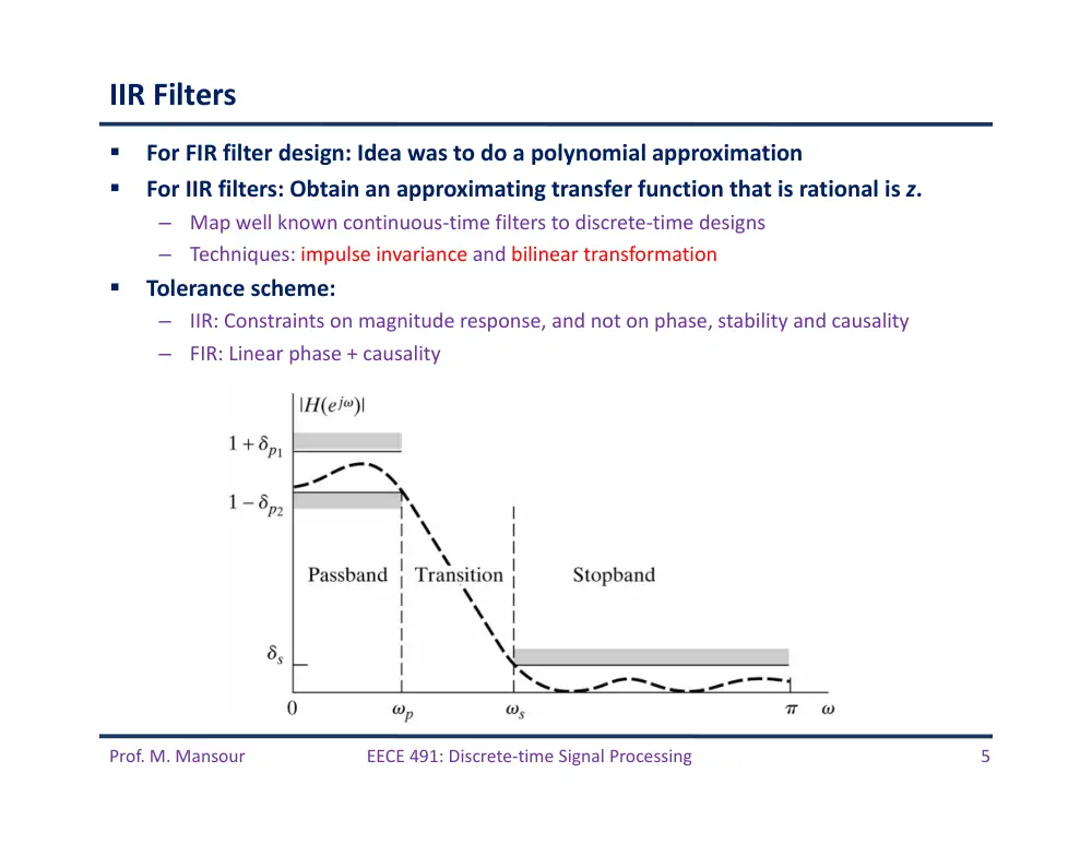Mansour EECE 491: Discrete‐time Signal Processing 5 IIR Filters  For FIR filter design: Idea was to do a polynomial approximation  For IIR filters: Obtain an approximating transfer function that is rational is z. – Map well known continuous‐time filters to discrete‐time designs – Techniques: impulse invariance and bilinear transformation  Tolerance scheme: – IIR: Constraints on magnitude response, and not on phase, stability and causality – FIR: Linear phase + causality Prof. M. 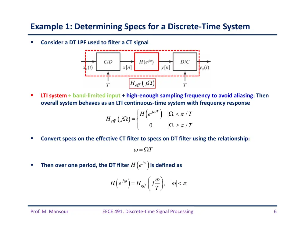Mansour EECE 491: Discrete‐time Signal Processing 6 Example 1: Determining Specs for a Discrete‐Time System  Consider a DT LPF used to filter a CT signal  LTI system + band‐limited input + high‐enough sampling frequency to avoid aliasing: Then overall system behaves as an LTI continuous‐time system with frequency response  Convert specs on the effective CT filter to specs on DT filter using the relationship:  Then over one period, the DT filter               is defined as     / 0 / j T eff H e T H j T              T     j  H e    , j eff H e H j T               Heff j Prof. M. 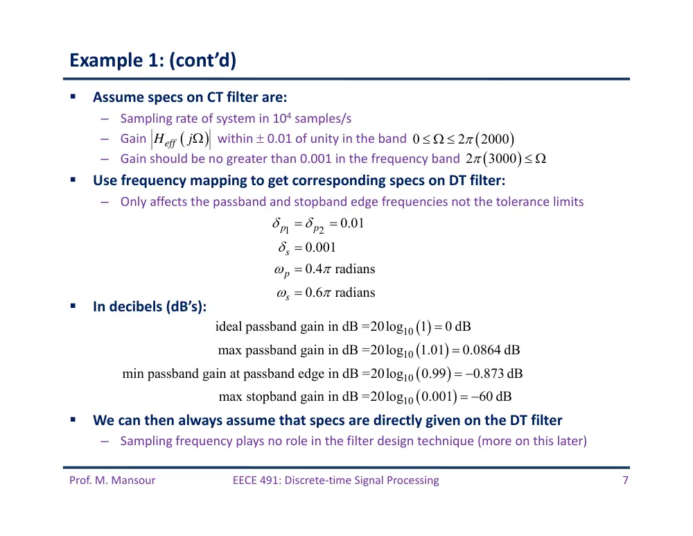Mansour EECE 491: Discrete‐time Signal Processing 7 Example 1: (cont’d)  Assume specs on CT filter are: – Sampling rate of system in 104 samples/s – Gain within  0.01 of unity in the band – Gain should be no greater than 0.001 in the frequency band  Use frequency mapping to get corresponding specs on DT filter: – Only affects the passband and stopband edge frequencies not the tolerance limits  In decibels (dB’s):  We can then always assume that specs are directly given on the DT filter – Sampling frequency plays no role in the filter design technique (more on this later)   Heff j   0 2  2000      2  3000   1 2 0.01 0.001 0.4 radians 0.6 radians p p s p s                     10 10 10 10 ideal passband gain in dB =20log 1 0 dB max passband gain in dB =20log 1.01 0.0864 dB min passband gain at passband edge in dB =20log 0.99 0.873 dB max stopband gain in dB =20log 0.001 60 dB       Prof. M. 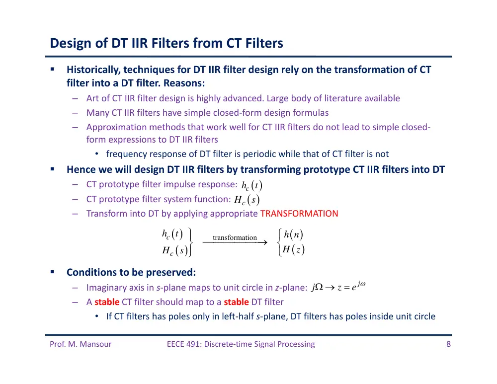Mansour EECE 491: Discrete‐time Signal Processing 8 Design of DT IIR Filters from CT Filters  Historically, techniques for DT IIR filter design rely on the transformation of CT filter into a DT filter. Reasons: – Art of CT IIR filter design is highly advanced. Large body of literature available – Many CT IIR filters have simple closed‐form design formulas – Approximation methods that work well for CT IIR filters do not lead to simple closed‐ form expressions to DT IIR filters • frequency response of DT filter is periodic while that of CT filter is not  Hence we will design DT IIR filters by transforming prototype CT IIR filters into DT – CT prototype filter impulse response: – CT prototype filter system function: – Transform into DT by applying appropriate TRANSFORMATION  Conditions to be preserved: – Imaginary axis in s‐plane maps to unit circle in z‐plane: – A stable CT filter should map to a stable DT filter • If CT filters has poles only in left‐half s‐plane, DT filters has poles inside unit circle ch   t Hc   s         transformation c c h t h n H z H s          j j z e     Prof. M. Mansour EECE 491: Discrete‐time Signal Processing 9 Review of Continuous‐Time Filters  Well‐known classes of CT filters: – Butterworth filter – Chebyshev filter – Elliptic filter Prof. M. 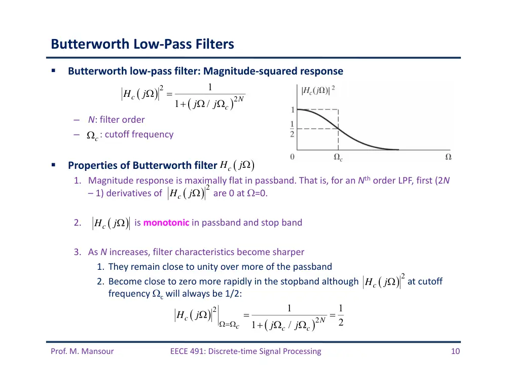Mansour EECE 491: Discrete‐time Signal Processing 10 Butterworth Low‐Pass Filters  Butterworth low‐pass filter: Magnitude‐squared response – N: filter order – : cutoff frequency  Properties of Butterworth filter 1. Magnitude response is maximally flat in passband. That is, for an Nth order LPF, first (2N – 1) derivatives of                      are 0 at =0. 2. is monotonic in passband and stop band 3. As N increases, filter characteristics become sharper 1. They remain close to unity over more of the passband 2. Become close to zero more rapidly in the stopband although                     at cutoff frequency c will always be 1/2:   Hc j   Hc j   2 Hc j     2 2 1 1 / c N c H j j j      c    2 Hc j     2 2 1 1 2 1 / c N c c c H j j j        Prof. M. Mansour EECE 491: Discrete‐time Signal Processing 11 Butterworth Low‐Pass Filters (cont’d) Prof. M. Mansour EECE 491: Discrete‐time Signal Processing 12 Butterworth Low‐Pass Filters (cont’d)  Poles of (roots of denominator) located on a circle of radius c at equally spaced points: – 2N poles equally spaced in angle on circle with radius c in s‐place, symmetrically located wrt imaginary axis – No pole falls on imaginary axis – N even: no pole falls on real axis – N odd: one pole falls on real axis – Angular spacing between poles is /N.           2 2 2 2 1 1 1 / 1 / c c c s j N N c c H s H s H j s j s                 2 2 1 / 2 1 , 0,1, , 1 N j k N c s e k N           N = 3 �� � �� ��   2 1 / /2 , 0,1, , 1 j k N j k c s e e k N          (and their symmetric points wrt imag axis) Prof. M. Mansour EECE 491: Discrete‐time Signal Processing 13 Butterworth Low‐Pass Filters (cont’d)  To determine              to associate with a LPF from – Factorize                     into – Poles of                             will always occur in pairs: pole at – Need to choose only one pole from each pair – To obtain a stable and causal filter, choose all poles in left‐half part of s‐plane  Example: for N = 3 – Choose poles at – Get – In general set numerator of              to        so that Hc   s   2 Hc j   2 Hc j     c c H s H s  Hc s  Hc s   s  sk  pole at s  sk sk  c, ce j2 /3, ce j2 /3 x x x Hc s   c 3 sc  sce j2 /3   s ce j2 /3   Hc s  c 3 Hc 0  1 Prof. M. Mansour EECE 491: Discrete‐time Signal Processing 14 Chebyshev Filters  In Butterworth filter: Magnitude response in monotonic in both passband and stopband – If filter specs are in terms on max passband and stopband approximation error, these specs are exceeded toward the low‐frequency end of passband and above the stopband cutoff frequency  More efficient approach leading to lower order filters – Distribute accuracy of approximation uniformly over passband or stopband or both – Achieved by choosing an approximation that has an equiripple behavior rather than a monotonic behavior  Class of Chebyshev filters achieve equiripple behavior – Type I Chebyshev filters: Equiripple in passband, monotonic in stopband – Type II Chebyshev filters: Monotonic in passband, equiripple in stopband Prof. M. Mansour EECE 491: Discrete‐time Signal Processing 15 Type I Chebyshev Filters  First few values:  Chebyshev polynomials are orthogonal and satisfy the recurrence:  For               ,             varies between 0 and 1  For x > 1, cos‐1(x) is imaginary and VN(x) behaves as a hyperbolic cosine, and hence increases monotonically     2 2 2 1 1 / c N c H j  V         1  cos cos VN x N  x  Type I Chebyshev Filter           0 1 1 1 2 2 1 cos cos cos 2cos 2 1 V x V x x x V x x x               1 1 2 N N N V x xV x V x     (Nth‐order Chebyshev polynomial) 0 1  x  2   VN x Prof. M. Mansour EECE 491: Discrete‐time Signal Processing 16 Type I Chebyshev Filters (cont’d)  For 0  /c  1:                  ripples between 1 and 1/(1 + 2)  For /c > 1:                  decreases monotonically  Parameters to be specified: , c, N. – : specified by allowable passband ripple – c: specified by desired passband cutoff frequency – Order N: chosen so that stopband specs are met.  Poles of Chebyshev filter: – Lie on an ellipse in s‐plane – Ellipse defined by 2 circles • Diameters = major & minor axes of ellipse     2 2 2 1 1 / c N c H j  V        2 Hc j   2 Hc j     1/ 1/ 1/ 1/ 1 2 1 length of minor axis : 2 , 2 1 length of major axis : 2 , 2 1 N N c N N c a a b b                     Prof. M. Mansour EECE 491: Discrete‐time Signal Processing 17 Type I Chebyshev Filters (cont’d)  To locate poles of Chebyshev filter – Identify points on major and minor circles equally spaced in angle with spacing /N. – Points are symmetrically located wrt imaginary axis – Point never falls on imaginary axis – A point occur on real axis for N odd, but not for N even. – Poles of filter then lie on ellipse • Ordinate specified by points identified on major circle • Abscissa specified by points identified on minor circle Prof. M. Mansour EECE 491: Discrete‐time Signal Processing 18 Type II Chebyshev Filters  Obtained from Type I Chebyshev filter via a transformation – Replace – To obtain  First design Type I filter, then apply transformation     2 2 2 2 1 / / N c N c V V            2 1 2 2 1 1 / c N c H j V            Prof. M. Mansour EECE 491: Discrete‐time Signal Processing 19 Elliptic Filters  Distribute error uniformly across both bandpass and stopband – Get equiripple both in passband and stopband – Best that can be achieved for a given filter order N. • That is, for given values of 1, 2, and p, the transition band s ‐ p is smallest  Elliptic filters have the form: – To obtain equiripple in both bands, elliptic filters must have both zeros and poles     2 2 2 1 1 c N H j  U      : Jacobian Elliptic Function UN  Filter has zeros on j‐axis in s‐plane Prof. M. Mansour EECE 491: Discrete‐time Signal Processing 20 Analog Filters in MATLAB  bilinear Bilinear transformation method for analog-to-digital filter conversion  besselap Bessel analog lowpass filter prototype  besself Bessel analog filter design  buttap Butterworth filter prototype  butter Butterworth filter design  cheb1ap Chebyshev Type I analog lowpass filter prototype  cheb2ap Chebyshev Type II analog lowpass filter prototype  cheby1 Chebyshev Type I filter design (passband ripple)  cheby2 Chebyshev Type II filter design (stopband ripple)  ellip Elliptic filter design  ellipap Elliptic analog lowpass filter prototype  freqs Frequency response of analog filters  lp2bp Transform lowpass analog filters to bandpass  lp2bs Transform lowpass analog filters to bandstop  lp2hp Transform lowpass analog filters to highpass  lp2lp Change cutoff frequency for lowpass analog filter Prof. M. Mansour EECE 491: Discrete‐time Signal Processing 21 Techniques for IIR Filter Design Design by Bilinear Transformation Prof. M. Mansour EECE 491: Discrete‐time Signal Processing 22 Filter Design by Impulse Invariance  DT system h[n] is defined by “sampling” the impulse response of a CT system hc(t) – DT impulse response corresponds to samples of the CT filter to be designed or simulated – DT system: h[n], H(z), H(ej) – CT system: hc(t), Hc(s), Hc(j)  In “impulse invariance” design, h[n] is chosen such that – Td: represents the sampling interval (does not play a role in the design procedure) – This transformation preserves the impulse response of the system at the sampled points  Relationship of CT and DT frequency responses H(ej) and Hc(j) – Sampling a CT signal leads to periodic replication in frequency domain – If CT filter is band‐limited, so that – Then     d c d h n T h nT    2 j c k d d H e H j j k T T                 0, / c d H j  T         , for j c Td H e H j         Prof. M. Mansour EECE 491: Discrete‐time Signal Processing 23 Filter Design by Impulse Invariance (cont’d)       1 s c s k H j H j k T         2 s d T      Hc j   Hs j Band‐limited    2 0, / N s N s N d c d T H j T                      , j c Td H e H j         Prof. M. Mansour EECE 491: Discrete‐time Signal Processing 24 Filter Design by Impulse Invariance (cont’d) – Related by a linear scaling of the frequency axis:  If CT filter is not band‐limited, then interference occurs, causing aliasing  If CT filter approaches zero at high frequencies, aliasing can then be negligible  When impulse‐invariance design procedure is used to utilize to CT filters to design DT filters with certain specs – Need to transform these specs to CT domain through the frequency relationship – Design the CT filter with these specs and then transform back to DT domain to get H(ej) – Sampling period in this case can’t be used to control aliasing. Need to over‐design the CT filter instead (to exceed the specs)   , j c d H e H j T             Td ,         CT filter is band-limited 0, / c d H j  T     /    Td Prof. M. Mansour EECE 491: Discrete‐time Signal Processing 25 Filter Design by Impulse Invariance (cont’d)  Impulse invariance was defined as a relation in time domain  What is the corresponding relation between the system functions Hc(s) and H(z)?  Assume a causal continuous‐time filer expressed in terms of partial fractions: – Corresponding impulse response (inverse Laplace): – Impulse response of causal DT filter is obtained by sampling – Therefore:     d c d h n T h nT    1 N k c k k A H s s s       1 0 0 0 N s t k k k c A e t h t t           d c   T h t           1 1 N s nT k d d c d d k k N n s T k d d k k h n T h nT T A e u n T A e u n            1 1 1 N d k s T k d k T A H z e z     Prof. M. Mansour EECE 491: Discrete‐time Signal Processing 26 Filter Design by Impulse Invariance (cont’d)  Pole at            in s‐plane maps to a pole                       in z‐plane  If real part of sk is negative so that CT filter is stable, then – Corresponding pole in z‐plane lies inside unit circle, and hence DT filter is stable  Zeros are not mapped in the same way  Hence, under impulse invariance mapping, the s‐plane is not similarly mapped to the z‐plane       1 1 1 1 N N k d k c s T k d k k k A T A H s H z s s e z          k s  s s T k d k z z e   1 s T e k d  Prof. M. Mansour EECE 491: Discrete‐time Signal Processing 27 Example: Impulse Invariance with a Butterworth Filter  Design a DT LPF by applying impulse invariance to a CT Butterworth filter  DT filter specs: – Passband gain between 0 dB and ‐1 dB – Stopband attenuation at least ‐15 dB  Note in the impulse invariance procedure, Td cancels out, so set it to 1 – Therefore the frequency mapping simply becomes  =   CT Butterworth filter specs  Magnitude of Butterworth filter is monotonic, then above constraints are satisfied if  Butterworth filter: Determine N and c:     0.89125 1, for 0 0.2 0.17783, for 0.3 j j H e H e               0.89125  Hc j   1, for 0    0.2 Hc j    0.17783, for 0.3           0 1 and 0.2 0.89125 0.3 0.17783 c c c H j H j H j          2 2 1 1 / c N c H j j j      2 2 2 2 0.2 1 1 0.89125 0.3 1 1 0..17783 N c N c                                   Prof. M. Mansour EECE 491: Discrete‐time Signal Processing 28 Example: Impulse Invariance with a Butterworth Filter  Get solution: – N = 5.8858 – c = 0.70474  Set N = 6 – Substitute back and get c = 0.7032  Magnitude square has 2N = 12 poles – Need to choose 6 in left half s‐plane – Pair 1 (s1, s1*): ‐0.182  j 0.679 – Pair 2 (s2, s2*): ‐0.497  j 0.497 – Pair 3 (s3, s3*): ‐0.679  j 0.182  Obtain H(z) by replacing poles at sk in s‐plane with poles at              6 * * * 1 1 2 2 3 3 2 2 2 0.12093 0.3640 0.4945 0.9945 0.4945 1.3585 0.4945 c Hc s s s s s s s s s s s s s s s s s s                sk k z z e   6th‐order Butterworth filter Prof. M. Mansour EECE 491: Discrete‐time Signal Processing 29 Example: Impulse Invariance with a Butterworth Filter   1 1 2 1 1 2 1 1 2 0.2871 0.4466 1 1.2686 0.7051 2.1428 1.1455 1 1.0691 0.3699 1.8557 0.6303 1 0.9972 0.2570 z H z z z z z z z z z                       Prof. M. Mansour EECE 491: Discrete‐time Signal Processing 30 Extensions of Impulse Invariance  In impulse invariance design, h[n] is chosen as – This transformation preserves the impulse response of the system  Can use other invariance criteria to do the transformation – Example: “Step‐invariance” – Assume CT filter has a step response of sc(t). Then the step‐response of the DT system s[n] is defined such that the “step response” remains invariant, i.e. s[n] = sc(nTd) • Obtain step response of CT system (sc(t) and its Laplace transform Sc(s)) • Sample sc(t) to obtain s[n] • Use the relationship between step response and impulse response to find h[n].  This way, if CT filter has good step response characteristics such as small rise time and low peak overshoot, they will be preserved in the DT filter  Concept can be extended to “waveform invariance”     d c d h n T h nT            1 1 s n h n u n H z S z z     Prof. M. Mansour EECE 491: Discrete‐time Signal Processing 31 Techniques for IIR Filter Design Design by Bilinear Transformation Prof. M. Mansour EECE 491: Discrete‐time Signal Processing 32 Bilinear Transformation  Algebraic relationship between s and z variables that maps entire j‐axis in s‐ plane into one revolution of unit circle in z‐plane – Map is not linear since – This map is used only when this warping of frequency axis is acceptable  Consider Hc(s) and H(z): – Bilinear map: replace s by – Td is included for historical reasons. Difference equation of H(z) can be obtained by applying trapezoidal integration rule to the differential equation corresponding to Hc(s) with Td as step size  Solving for z:  Substituting s =  + j:              1 1 2 1 1 d z s T z                1 1 2 1 1 c d z H z H T z                           1 / 2 1 / 2 d d T s z T s    1 / 2 / 2 1 / 2 / 2 d d d d T j T z T j T          Prof. M. Mansour EECE 491: Discrete‐time Signal Processing 33 Bilinear Transformation  If  < 0 then |z| < 1 for any  , and if  > 0 then |z| > 1 for any  – Pole in left‐half s‐plane maps inside unit circle in z‐plane – Therefore, a causal and stable CT filter maps to a causal and stable DT filter  To show that entire j‐axis in s‐plane maps unit circle in z‐plane, let  = 0, then – Hence |z| = 1 for any . Then falls on unit circle and takes the form 1 / 2 / 2 1 / 2 / 2 d d d d T j T z T j T          1 / 2 1 / 2 d d j T z j T      1 / 2 1 / 2 j d d j T e j T       Prof. M. Mansour EECE 491: Discrete‐time Signal Processing 34 Bilinear Transformation Prof. M. Mansour EECE 491: Discrete‐time Signal Processing 35 Bilinear Transformation: Relationship Between  and   1 1 2 1 2 1 , 1 1 j j j d d z e s z e s T T z e                                      /2 /2 2 sin / 2 2 2 tan / 2 2 cos / 2 j j d d e j j s j j T T e                              2 0 tan / 2 or 2arctan d / 2 d T T          Prof. M. Mansour EECE 491: Discrete‐time Signal Processing 36 Frequency Warping of Bilinear Transformation • Frequency warping inherent in the bilinear transformation of a continuous‐time lowpass filter into a discrete‐time lowpass filter. • To achieve the desired discrete‐time cutoff frequencies, the continuous‐ time cutoff frequencies must be pre‐ warped as indicated. • Bilinear transformation is useful when this non‐linearity is tolerable as in the case of filters that approximate ideal piecewise‐constant magnitude response characteristics Prof. M. Mansour EECE 491: Discrete‐time Signal Processing 37 Distortion of Phase Response  Apply bilinear transformation to linear phase factor – Get DT phase angle of linear phase phase resulting from bilinear transformation e s       2 / tan / 2  Td   Prof. M. Mansour EECE 491: Discrete‐time Signal Processing 38 Example: Bilinear Transformation of a Butterworth Filter  Design a DT LPF by applying bilinear transformation to a CT Butterworth filter  DT filter specs: – Passband gain between 0 dB and ‐1 dB – Stopband attenuation at least ‐15 dB  CT Butterworth filter specs (choose Td = 1)  Magnitude of Butterworth filter is monotonic, then above constraints are satisfied if  Butterworth filter: Determine N and c:     0.89125 1, for 0 0.2 0.17783, for 0.3 j j H e H e                       0.89125 1, for 0 2tan 0.2 / 2 0.17783, for 2tan 0.3 / 2 c c H j H j                         0 1 and 2tan 0.1 0.89125 2tan 0.15 0.17783 c c c H j H H j          2 2 1 1 / c N c H j j j          2 2 2 2 2tan 0.1 1 1 0.89125 2tan 0.15 1 1 0.17783 N c N c                                       2 tan / 2 2tan / 2 Td      • Get N = 5.305 • Round to N = 6 • Substitute to get c=0.766 Prof. M. Mansour EECE 491: Discrete‐time Signal Processing 39 Example: Bilinear Transformation of a Butterworth Filter  In s‐plane, there are 12 poles – Choose 6 pole‐pairs in left‐half s‐plane – Apply bilinear transformation with Td = 1 to get H(z):       2 2 2 0.20238 0.3996 0.5871 1.0836 0.5871 1.4802 0.5871 Hc s s s s s s        1 1 2 1 1 z s z                      6 1 1 2 1 2 1 2 0.0007378 1 1 1.2686 0.7051 1 1.0106 0.3583 1 0.9044 0.2155 z H z z z z z z z                Prof. M. Mansour EECE 491: Discrete‐time Signal Processing 40 Example: Bilinear Transformation of a Butterworth Filter Prof. M. Mansour EECE 491: Discrete‐time Signal Processing 41 Design Comparisons  Design a DT filter by applying Bilinear transformation to Butterworth, Chebyshev Type I and II, and Elliptic filters  DT filter specs: Meet or exceed the following passband edge frequency 0.5 radians stopband edge frequency 0.6 radians max passband gain 0 dB min passband gain 0.3 dB max stopband gain 30 dB p s                  10 1 1 10 1 2 10 20log 1 0 dB 0 20log 1 0.3 dB 0.0339 20log 30 dB 0.0316 p p p p s s                    Prof. M. Mansour EECE 491: Discrete‐time Signal Processing 42 Butterworth Filter: 15th‐Order Prof. M. Mansour EECE 491: Discrete‐time Signal Processing 43 Chebyshev Type I Filter: 7th‐order Prof. M. Mansour EECE 491: Discrete‐time Signal Processing 44 Chebyshev Type II Filter: 7th‐order Prof. M. Mansour EECE 491: Discrete‐time Signal Processing 45 Elliptic Filter: 5th‐order, Exceeds Design Specifications Prof. M. Mansour EECE 491: Discrete‐time Signal Processing 46 Elliptic Filter: 5th‐order, Exceeds Design Specifications