
EECE 491 Lecture 3, Spring 2016
American University of Beirut · Discrete-time Signal Processing · 79 pages · Prof. Mohammad Mansour

Showing the first 10 of 79 pages. Download the PDF to see all of it.
More EECE 491 files
Show the text of this lab
Prof. M. Mansour
EECE 491: Discrete‐time Signal Processing
1
EECE 491: Discrete‐time Signal Processing
Mohammad M. Mansour
Dept. of Electrical and Compute Engineering
American University of Beirut
Lecture 3: Discrete‐time Signal and Systems
Prof. M. Mansour
EECE 491: Discrete‐time Signal Processing
2
Announcements
Reading
–
Chapter 2, Proakis
Prof. M. Mansour
EECE 491: Discrete‐time Signal Processing
3
Outline
DT Signals
DT Systems
Analysis of DT LTI Systems
DT Systems Described by Difference Equations
Implementation of DT Systems
Correlation of DT Signals
Prof. M. Mansour
EECE 491: Discrete‐time Signal Processing
4
I ‐ Discrete‐Time Signals
Prof. M. Mansour
EECE 491: Discrete‐time Signal Processing
5
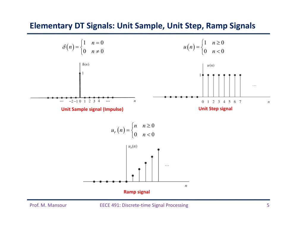
Elementary DT Signals: Unit Sample, Unit Step, Ramp Signals
1
0
0
0
n
n
n
1
0
0
0
n
u n
n
0
0
0
r
n
n
u
n
n
Unit Sample signal (Impulse)
Unit Step signal
Ramp signal
Prof. M. Mansour
EECE 491: Discrete‐time Signal Processing
6
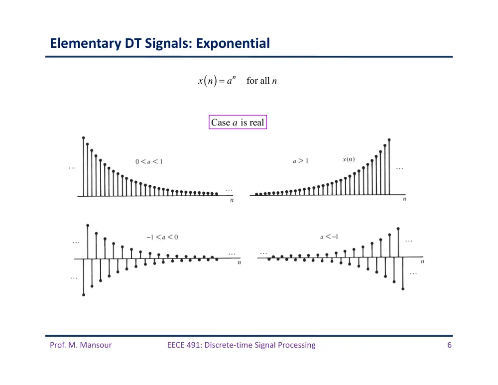
Elementary DT Signals: Exponential
for all
n
x n
a
n
Case is real
a
Prof. M. Mansour
EECE 491: Discrete‐time Signal Processing
7
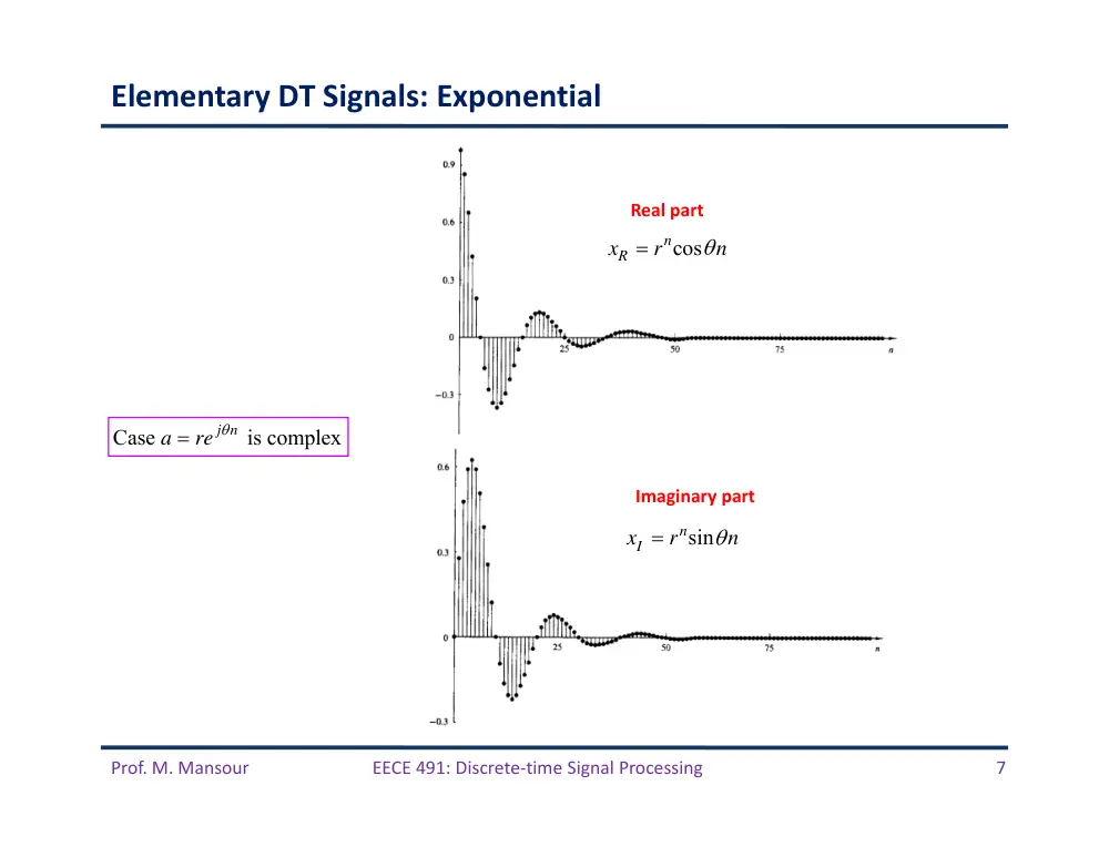
Elementary DT Signals: Exponential
Case
j n is complex
a
re
Real part
Imaginary part
ncos
xR
r
n
nsin
Ix
r
n
Prof. M. Mansour
EECE 491: Discrete‐time Signal Processing
8
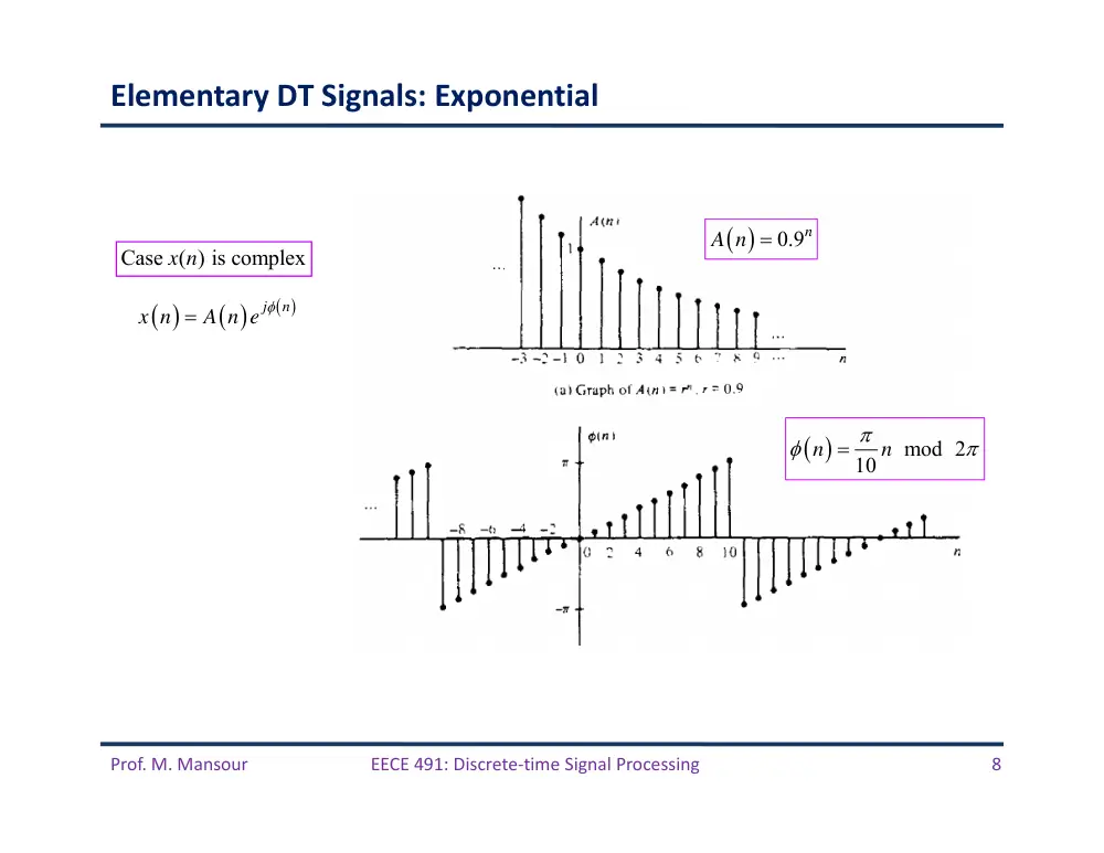
Elementary DT Signals: Exponential
Case ( ) is complex
x n
j
n
x n
A n e
0.9n
A n
mod 2
10
n
n
Prof. M. Mansour
EECE 491: Discrete‐time Signal Processing
9
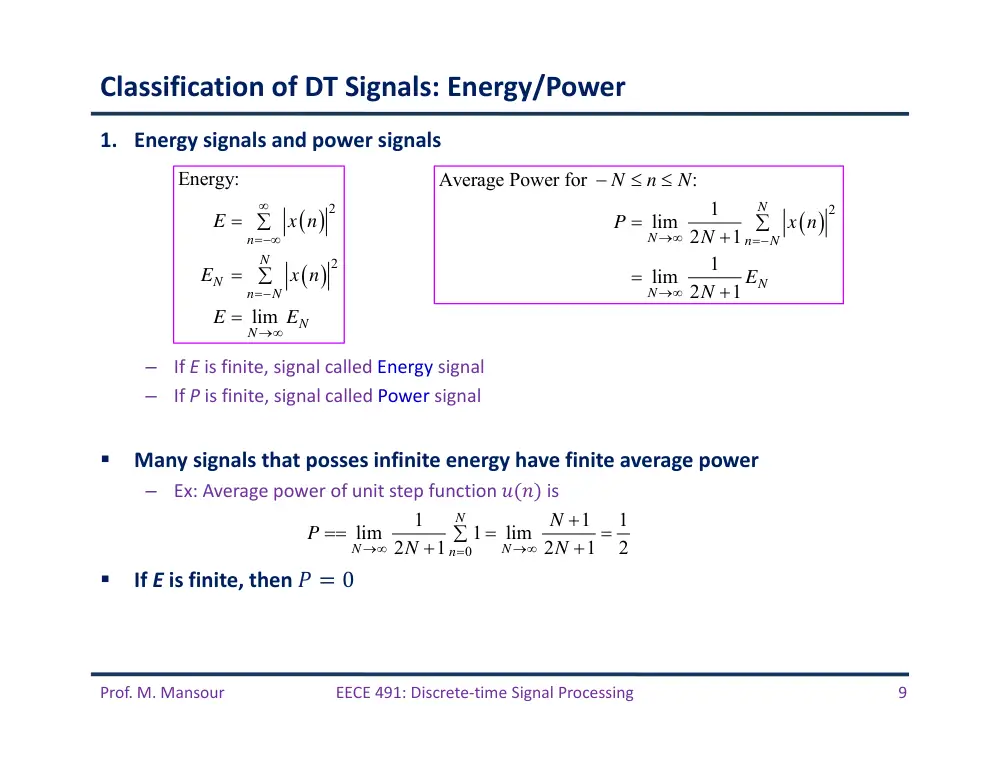
Classification of DT Signals: Energy/Power
1. Energy signals and power signals
–
If E is finite, signal called Energy signal
–
If P is finite, signal called Power signal
Many signals that posses infinite energy have finite average power
–
Ex: Average power of unit step function ���� is
If E is finite, then � � 0
2
2
Energy:
lim
n
N
N
n
N
N
N
E
x n
E
x n
E
E
2
Average Power for
:
1
lim 2
1
1
lim 2
1
N
N
n
N
N
N
N
n
N
P
x n
N
E
N
0
1
1
1
lim
1
lim
2
1
2
1
2
N
N
N
n
N
P
N
N
Prof. M. Mansour
EECE 491: Discrete‐time Signal Processing
10
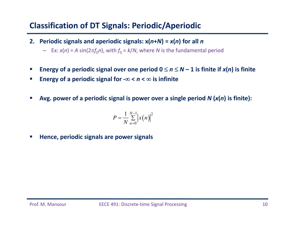
Classification of DT Signals: Periodic/Aperiodic
2. Periodic signals and aperiodic signals: x(n+N) = x(n) for all n
–
Ex: x(n) = A sin(2f0n), with f0 = k/N, where N is the fundamental period
Energy of a periodic signal over one period 0 n N – 1 is finite if x(n) is finite
Energy of a periodic signal for ‐ < n < is infinite
Avg. power of a periodic signal is power over a single period N (x(n) is finite):
Hence, periodic signals are power signals
1
2
0
1 N
n
P
x n
N
Prof. M. Mansour
EECE 491: Discrete‐time Signal Processing
11
Classification of DT Signals
3. Symmetric (even) and anti‐symmetric (odd) signals:
–
Even iff: x(‐n) = x(n)
–
Odd iff: x(‐n) = ‐x(n). Hence x(0) = 0
For an arbitrary signal x(n), we can express its even and odd parts as:
Even
Odd
1
2
1
2
e
o
x
n
x n
x
n
x
n
x n
x
n
Prof. M. Mansour
EECE 491: Discrete‐time Signal Processing
12
Time‐Shifting Operation
Shifting by k time units:
x n
x n
k
Prof. M. Mansour
EECE 491: Discrete‐time Signal Processing
13
Time‐Shifting Operation: Example
Consider the DT signal below. Write down an equation describing p(n)
Answer: p(n) can be represented as a sum of 4 scaled and delayed impulses:
3
1
2
7
3
1
2
7
p n
a
n
a
n
a
n
a
n
Prof. M. Mansour
EECE 491: Discrete‐time Signal Processing
14
Folding Operation
Note: Folding shifting are not
commutative
Fold then shift x(n) by k:
Shift x(n) by k then fold:
x n
x
n
1y
n
x
n
k
y2
n
x
n
k
Prof. M. Mansour
EECE 491: Discrete‐time Signal Processing
15
Time‐Shifting and Folding: Example
Example: Form the sequence h(k – n) from h(n) .
The sequence h(n) as a function of �.
The sequence h(–n) as a function of �.
The sequence h(k–n) = h(–(n – k)) as a function of n for k = 4.
�
�
h n
1
0
h n
h
n
h
n
2
1
h
n
h n
k
h k
n
h
n
k
Prof. M. Mansour
EECE 491: Discrete‐time Signal Processing
16
Down‐Sampling Operation
where � is an integer
decrease sampling rate by 2x
x n
x
n
Prof. M. Mansour
EECE 491: Discrete‐time Signal Processing
17
Discrete‐Time Systems
Prof. M. Mansour
EECE 491: Discrete‐time Signal Processing
18
Input‐Output Description of Systems
Example: Determine the response of the following systems to the input signal
3
3
ˆ
0,0,3,2,1,0,1,2,3,0,0,
0
otherwise
n
n
x n
1
ˆ
:
,3,2,1,0,1,2,3,0,
y n
x n
A y n
1
1
1
3
ˆ
5
2
5
:
,0,1,
,2,1,
,1,2,
,1,0
3
3
3
y n
x n
x n
x n
A y n
(moving average filter)
1
1
ˆ
:
0,2,2,1,1,1,2,2,0,0,0,
y n
median x n
x n
x n
A y n
(median filter)
1
2
ˆ
:
,0,3,5,6,6,7,9,12,12,
n
k
y n
x k
x n
x n
x n
A y n
(accumulator)
Prof. M. Mansour
EECE 491: Discrete‐time Signal Processing
19
Example: Moving Average with Window of 6 Samples
2
2
1
2
1
1
1
,
1
M
k M
y n
x n
k
M
M
M
M
����
�
Prof. M. Mansour
EECE 491: Discrete‐time Signal Processing
20
Initial Conditions
For the accumulator function:
Example: Let x(n) = nu(n). Find y(n) assuming y(–1) = 0
Solution:
Example: Find y(n) assuming y(2) = 1
1
n
k
y n
x n
y n
x n
requires 1 initial condition
1
0
0
1
1
1
1
2
2
n
n
k
k
k
n
k
y n
x n
x k
x k
y
k
n n
n n
y
2
3
3
2
1
1
1
3
2
2
2
n
k
k
n
k
y n
x k
x k
y
k
n n
n n
Prof. M. Mansour
EECE 491: Discrete‐time Signal Processing
21
Block Diagram Representation of DT Systems
signal adder
constant multiplier
signal multiplier
unit delay
unit advance
Prof. M. Mansour
EECE 491: Discrete‐time Signal Processing
22
Example
What is the input‐output relationship that the following block diagram
implements?
1
1
1
1
1
4
2
2
y n
y n
x n
x n
Prof. M. Mansour
EECE 491: Discrete‐time Signal Processing
23
Time‐Varying vs. Time‐Invariant Systems
Time‐invariant (TI): Input‐output characteristics do not change with time
–
Assume system produces an output y(n) when excited with input signal x(n)
–
Now assume input is delayed by k time units and then applied to system. If the system
characteristics do not change, the system should produce the same response as that to
x(n) but delayed by k time units.
In general, delaying x(n) by k time units and applying it to system, we get
–
If
for all possible shift values of k, system in TI
–
If
even for one value of k, system is time‐varying
H
H
x n
y n
x n
k
y n
k
LTI
for every input ���� and time shift �
,
y n k
H x n
k
,
y n k
y n
k
,
y n k
y n
k
Prof. M. Mansour
EECE 491: Discrete‐time Signal Processing
24
Example
Determine which of the following systems are TI or time‐varying.
1
,
1
y n
x n
x n
y n k
x n
k
x n
k
y n
k
,
y n
nx n
y n k
nx n
k
y n
k
n
k x n
k
,
y n
x
n
y n k
x
n
k
y n
k
x
n
k
0
0
0
cos
,
cos
cos
y n
x n
n
y n k
x n
k
n
y n
k
x n
k
n
k
Prof. M. Mansour
EECE 491: Discrete‐time Signal Processing
25
Linear vs. Non‐Linear Systems
A linear system is one that satisfies the superposition principle
1 1
2 2
1
1
2
2
H a x
n
a x
n
a H x
n
a H x
n
Prof. M. Mansour
EECE 491: Discrete‐time Signal Processing
26
Example
Which of the following systems are linear and which are non‐linear.
1.
y(n) = n x(n)
2.
y(n) = x(n2)
3.
y(n) = x2(n)
4.
y(n) = Ax(n) + B
5.
y(n) = ex(n)
1
1
2
2
3
1 1
2
2
1
1
2
2
1 1
2
2
,
y
n
nx
n
y
n
nx
n
y
n
n a x
n
a x
n
a nx
n
a nx
n
a y
n
a y
n
2
2
1
1
2
2
2
2
3
1 1
2
2
1 1
2
2
,
y
n
x
n
y
n
x
n
y
n
a x
n
a x
n
a y
n
a y
n
linear
linear
2
2
1
1
2
2
2
2
2
3
1 1
2
2
1 1
2
2
1 1
2
2
,
y
n
x
n
y
n
x
n
y
n
a x
n
a x
n
a y
n
a y
n
a x
n
a x
n
nonlinear
1
2
3
1 1
2
2
1 1
2
2
1
2
1
2
1
2
,
y
n
Ax
n
y
n
Ax
n
y
n
A a x
n
a x
n
a y
n
a y
n
a
Ax
n
a
Ax
n
B
B
B
B
B
1
2
1
2
1 1
2 2
1
2
3
1 1
2
2
1
2
x n ,
x
n
a x n
a x
n
x n
x
n
y
n
e
y
n
e
y
n
e
a y
n
a y
n
a e
a e
nonlinear
nonlinear
Prof. M. Mansour
EECE 491: Discrete‐time Signal Processing
27
Causal vs Non‐Causal Systems
If the output of system at any time n depends only on current and past inputs [i.e. x(n), x(n‐
1), … ] but does not depend on future inputs [i.e. x(n+1), x(n+2), … ], it is called causal.
Examples:
–
y(n) = x(n) – x(n – 1)
–
y(n) = a x(n)
–
y(n) = x(n) + 3 x(n + 4)
–
y(n) = x(n2)
–
y(n) = x(2n)
–
y(n) = x(‐n)
causal
causal
causal
non‐causal
non‐causal
non‐causal
non‐causal
n
k
y n
x k
Prof. M. Mansour
EECE 491: Discrete‐time Signal Processing
28
Stable vs. Unstable Systems
Bounded‐Input, Bounded‐Output (BIBO) Stability
–
A system is BIBO stable if every bounded‐input produces a bounded output
Hence there exist some finite numbers �� and �� such that
Example: Is the system with IO relation
BIBO stable?
Solution: If we excite the system with x(n) = C(n) (which is bounded) where C > 1
is a constant, then we obtain the following outputs assuming y(‐1) = 0:
–
y(0) = C
–
y(1) = C2
–
y(2) = C4
–
…
–
y(n) = C2n
Hence system is not BIBO stable
,
x
y
x n
M
y n
M
2
1
y n
y
n
x n
Prof. M. Mansour
EECE 491: Discrete‐time Signal Processing
29
Interconnection of DT Systems
Cascade (series): In general, order matters
–
For LTI systems T1 and T2, order does not matter and combined T1T2 system is LTI. Proof?
Parallel
Prof. M. Mansour
EECE 491: Discrete‐time Signal Processing
30
Analysis of Discrete‐time LTI Systems
Prof. M. Mansour
EECE 491: Discrete‐time Signal Processing
31
Techniques for Analyzing Linear Systems
Main theme:
–
Any input signal can be decomposed and represented as a weighted sum of impulses
–
LTI systems are fully characterized by their response to a unit sample (impulse)
sequence.
Methods to determine behavior of LTI system
–
Method 1: Directly solve the input‐output equation describing the system
–
Method 2: Resolve input into weighted sum of impulses, get response to an impulse,
then use linearity and time‐invariance properties of system to get response of arbitrary
input
General form of input‐output relationship for an LTI system
–
Called difference equation
–
Function of N past outputs, each weighted by ak.
–
Function of current and M past inputs, each weighted by bk.
1
0
N
M
k
k
k
k
y n
a y n
k
b x n
k
Prof. M. Mansour
EECE 491: Discrete‐time Signal Processing
32
Resolution of a DT Signal into Impulses
k
x n
x k
n
k
Prof. M. Mansour
EECE 491: Discrete‐time Signal Processing
33
Response of Linear Systems to Arbitrary Inputs: Convolution Sum
Denote response y(n,k) of system to the input impulse at n = k by the special
symbol h(n,k), for – < k <
If the input impulse is scaled by x(k), response is scaled as x(k)h(n,k) as well
If
, then the response is the corresponding sum of
weighted outputs:
The above response is for any linear system (not necessarily LTI)
–
We only used the linearity or superposition property, but not time‐invariance property
,
,
y n k
h n k
n
k
T
time index
location of impulse
,
,
k
k
k
y n k
x n
x k
n
k
x k
n
k
x k h n k
T
T
T
applies for any linear system
called impulse response function
k
x n
x k
n
k
Prof. M. Mansour
EECE 491: Discrete‐time Signal Processing
34
If System is Linear + Time‐Invariant ….
Notes:
–
LTI system is completely characterized by h(n)
–
Otherwise, a time‐varying system requires knowledge of an infinite number of impulse
response functions h(n,k), one for each delay k.
–
Convolution sum is commutative in x and h
How to obtain the response at a particular time instant n = n0?
h n
n
T
time invariance
h n
k
n
k
T
,
,
k
y n k
x k h n k
k
y n
x k h n
k
… Convolution Sum
0
0
k
y n
x k h n
k
k
k
y n
x k h n
k
h k x n
k
y n
x n
h n
Prof. M. Mansour
EECE 491: Discrete‐time Signal Processing
35
Graphical Computation of Convolution Sum
Example
–
� � � 1, 2�, 1, �1
–
� � � 1�, 2, 3, 1
0
0
k
y n
x k h n
k
Prof. M. Mansour
EECE 491: Discrete‐time Signal Processing
36
Graphical Computation of Convolution Sum (Example cont’d)
Prof. M. Mansour
EECE 491: Discrete‐time Signal Processing
37
Example
Determine y(n) of an LTI system with impulse response
when the input is a unit step sequence x(n) = u(n)
,
1
n
h n
a u n
a
Prof. M. Mansour
EECE 491: Discrete‐time Signal Processing
38
Example (cont’d)
2
2
1
1
1
1
n
y n
a
a
a
a
a
for
0
n
y n 0
for
n 0
Prof. M. Mansour
EECE 491: Discrete‐time Signal Processing
39
Properties of Convolution
Commutativity:
Associativity:
y n
x n
n
x n
x n
n
k
y n
k
x n
k
y n
x n
h n
h n
x n
1
2
1
2
x n
h
n
h
n
x n
h n
h
n
Prof. M. Mansour
EECE 491: Discrete‐time Signal Processing
40
Example
Determine impulse response for the cascade of 2 LTI systems with
Solution:
Hence for n k 0, we have
1
2
1
2
1
4
n
n
h
n
u n
h
n
u n
1
2
k
h n
h
k h
n
k
0
0
1
1
2
4
1
4
1
1
2
2
2
2
,
0
k
n k
n
n
n
n
k
n
k
k
h n
n
1
2
h n
h
n
h
n
1
2
0
0 or
0
1
1
0
0
2
4
k
n k
k
n
k
h k h
n
k
n
Prof. M. Mansour
EECE 491: Discrete‐time Signal Processing
41
Properties of Convolution (cont’d)
Distributive law
1
2
1
2
x n
h n
h
n
x n
h n
x n
h
n
Prof. M. Mansour
EECE 491: Discrete‐time Signal Processing
42
Causal LTI Systems
For LTI systems, causality can be translated into a condition on h(n)
Causal LTI h(n) = 0 for n < 0
Two equivalent forms:
If the input is a causal sequence, i.e., x(n) = 0 for n < 0, then convolution
becomes:
0
0
1
0
0
0
k
k
k
y n
h k x n
k
h k x n
k
h k x n
k
current & past values
future values
Causal 0
k 0
n
k
y n
h k x n
k
x k h n
k
0
0
n
k
n
k
y n
h k x n
k
x k h n
k
Prof. M. Mansour
EECE 491: Discrete‐time Signal Processing
43
Example
Determine the unit step response of the LTI system with impulse response
Solution: Since h(n) is causal, and x(n) = u(n) is causal, then
,
1
n
h n
a u n
a
1
0
1
for
0
1
( )
0
for
0
n
n
k
k
a
y n
a
n
a
y n
n
Prof. M. Mansour
EECE 491: Discrete‐time Signal Processing
44
Stability of LTI Systems
An LTI system is BIBO stable if and only if h[n] is absolutely summable:
h
k
S
h k
Prof. M. Mansour
EECE 491: Discrete‐time Signal Processing
45
Finite‐Duration and Infinite‐Duration Impulse Response
Finite‐Impulse Response (FIR) of order �:
Hence FIR system operates on a window of only the most recent � values of x(n)
Infinite‐Impulse Response (IIR): Has infinite duration impulse response
0,
0
and
h n
n
n
M
1
0
M
k
y n
h k x n
k
⇒ convolution sum becomes
0
k
y n
h k x n
k
(causality assumed)
system has infinite memory
Prof. M. Mansour
EECE 491: Discrete‐time Signal Processing
46
DT Systems Described by Difference Equations
Prof. M. Mansour
EECE 491: Discrete‐time Signal Processing
47
Recursive and Non‐recursive DT Systems
Can a system described by the input‐output relationship below be implemented?
Clearly, for FIR case, it is possible
What bout IIR case?
–
If we can express the current output in terms of current and past inputs, as well as past
outputs, then such a system can be physically realized
–
This class of LTI IIR systems that can be expressed in terms of difference equations is
physically realizable
Example: Cumulative average system
–
Memory grows with �
–
We can express as a recursion
0
k
y n
h k x n
k
0
1
,
0,1,2,
1
n
k
y n
x k
n
n
1
1
1
1
n
y n
y n
x n
n
n
Prof. M. Mansour
EECE 491: Discrete‐time Signal Processing
48
Example: Square‐Root Algorithm
Calculators implement square‐root of � � � using the iterative algorithm
The following recursive system when excited with x(n) = Au(n) with appropriate
initial condition, the response will converge toward as � increases
–
We do not need to specify an exact initial condition y(‐1). A rough estimate is enough
1
1
1
,
0,
0,1,2,
2
n
n
n
A
s
s
A
n
s
1
1
2
1
A
y n
y n
y n
A
Prof. M. Mansour
EECE 491: Discrete‐time Signal Processing
49
Recursive and Non‐recursive DT Systems
Basic form of causal and realizable non‐recursive and recursive systems
Non‐recursive
Recursive
Prof. M. Mansour
EECE 491: Discrete‐time Signal Processing
50
LTI Systems with Constant‐Coefficient Difference Equations
Systems described by constant‐coefficient difference equations are LTI systems:
Principle of linearity results in:
–
Total response is the sum of the zero‐input and zero‐state responses:
–
Zero‐input response: Solve for y(n) when x(n) = 0
–
Zero‐state response: Solve for y(n), n ≥ 0, when y(‐1) = 0.
1
0
N
M
k
k
k
k
y n
a y n
k
b x n
k
zi
zs
y n
y
n
y
n
Prof. M. Mansour
EECE 491: Discrete‐time Signal Processing
51
Solution of Linear Constant‐Coefficient Difference Equations
Goal is to determine output y(n), n 0, of system given a specific input x(n), n 0,
and a set of initial conditions
Solution composed of homogeneous solution yh(n) and particular solution yp(n)
yh(n): solution to the homogeneous difference equation
Form characteristic polynomial: Solution is in the form of an exponential, yh(n)=n
–
Solution has N roots, :
Coefficients are determined from the initial conditions of the system
–
Result gives zero‐input response yzi(n)
1
0
N
M
k
k
k
k
y n
a y n
k
b x n
k
h
p
y n
y
n
y
n
0
0
0,
1
N
k
k
a y n
k
a
0
0
N
n k
k
k
a
1 1
2
2
n
n
n
h
N
N
y
n
C
C
C
≥
≥
λ1 … λN
Prof. M. Mansour
EECE 491: Discrete‐time Signal Processing
52
Solution of Linear Constant‐Coefficient Difference Equations
Particular solution: Solution yp(n) required to satisfy DE for the specific input x(n)
yp(n) is any solution satisfying
We assume yp(n) has a form that depends on the form of the input x(n)
yp(n) is the limiting value of the zero‐state response: (steady‐state response)
0
1
0
,
1
N
M
k
p
k
k
k
a y
n
k
b x n
k
a
lim
p
zs
n
y
n
y
n
Prof. M. Mansour
EECE 491: Discrete‐time Signal Processing
53
Example
Determine solution of the system described by the first‐order DE when x(n) = u(n):
Solution:
–
Homogeneous solution: set x(n) = 0. The assumed solution has the form yh(n)=n
–
To get zero‐input response, find coefficient �. Use initial conditions of the system ���1�
–
When ���� � 0, we have ��0� � �1���1�.
–
Also, ���0� � �
–
Therefore,
–
Particular solution when ���� � ����: Assume ����� also has the form ����� � �����
–
Substitute in DE:
• Evaluate for any � � 1 where none of the terms vanish:
1
1
1
,
1
y n
a y n
x n
a
1
1
1
1
1
0
n
n
n
a
a
a
1
n
n
yh
n
C
C
a
1
1
1
n
yzi
n
a
y
1
1
Ku n
a Ku n
u n
1
1
1
1
1
K
a K
K
a
1
1
1
yp
n
a u n
Prof. M. Mansour
EECE 491: Discrete‐time Signal Processing
54
Example (cont’d)
Total solution:
The constant is determined to satisfy the initial condition �����. For example, to
determine the zero‐state response, set � �� � � and evaluate DE at � � 0.
To get � for any � �� , we evaluate DE at � � 0
On the other hand:
Therefore
Substitute back in total solution:
1
1
1
,
0
1
n
y n
C
a
n
a
1
1
1
1
0
1
0
0
1
1
y n
a y n
u n
y
a y
u
y
a y
0
1
1
1
1
1
0
1
1
y
C
a
C
a
a
1
1
1
1
1
a
C
a y
a
1
1
1
1
1
1
1
,
0
1
n
n
zi
zs
a
y n
a
y
n
a
y
n
y
n
Prof. M. Mansour
EECE 491: Discrete‐time Signal Processing
55
Example
Determine the particular solution of the DE when ���� � ������:
Solution: ����� � �������
To determine �, evaluate above equation for any � � �
5
1
1
2
6
6
y n
y n
y n
x n
1
2
5
1
2
2
1
2
2
2
6
6
n
n
n
n
K
u n
K
u n
K
u n
u n
2
1
0
2
5
1
8
2
2
2
2
6
6
5
K
K
K
K
8 2
5
n
yp
n
u n
Prof. M. Mansour
EECE 491: Discrete‐time Signal Processing
56
Example
Determine the response ���� for � � � of the system described by the second‐order DE
when ���� � ������:
Solution: Homogeneous part has the form �� � � ��
–
To get zero‐input solution, use initial conditions ���1� and ���2� of the system:
•
� 0 � 3� �1 � 4� �2 � �� � ��
•
� 1 � 3� 0 � 4� �1 � 13� �1 � 12� �2 � ��� � 4��
•
∴ �� � �
�
� � �1 �
�
� � �2 , ���
��
� � �1 �
��
� � �2
3
1
4
2
2
1
y n
y n
y n
x n
x n
1
2
2
2
1
2
3
4
3
4
0
1,
4
n
n
n
n
1 1
2
2
1
2
1
4
n
n
n
n
yh
n
C
C
C
C
1
4
16
16
1
2
1
1
2
4
,
0
5
5
5
5
n
n
yzi
n
y
y
y
y
n
Prof. M. Mansour
EECE 491: Discrete‐time Signal Processing
57
Example (cont’d)
Particular solution when ���� � 4�����: Assume ����� also has the form ����� � �4�����
Observe that this particular solution is already included in the homogeneous solution
We select the particular solution to be linearly independent of the homogeneous part
Substitute back in DE and evaluate for � � �, we get � � �
�
Total solution:
Next, determine the zero‐state response (���1� � ���2� � 0). From DE, we have
–
� 0 � 3� �1 � 4� �2 � 1 � 1 � �� � ��
–
� 1 � 3� 0 � 4� �1 � 6 � 13� �1 � 12� �2 � 9 � 9 � ��� � 4�� �
��
�
–
Get �1 � �
�
�� and �2 �
��
��
4n
yp
n
Kn
u n
6 4
5
n
yp
n
n
u n
1
2
6
1
4
4
5
n
n
n
y n
C
C
n
u n
1
26
6
1
4
4
25
25
5
n
n
n
yzs
n
n
u n
Prof. M. Mansour
EECE 491: Discrete‐time Signal Processing
58
Impulse Response of LTI Recursive Systems
Step response: Response to � � � ����
Impulse response ����: Response to � � � ����
In case of a recursive system, ���� is the zero‐state response to � � � ���� and
system is initially at rest
Example: � � � �� � � � � ����
General case:
1
0
0
1
,
0
,
0
,
0
n
n
k
k
n
k
zs
k
n
y n
a
y
a x n
k
n
y
n
a
n
k
n
a
n
n
h n
a u n
0
0
,
0
,
0
n
zs
k
n
k
y
n
h k x n
k
n
h k
n
k
n
h n
Prof. M. Mansour
EECE 491: Discrete‐time Signal Processing
59
Example
Determine the impulse response of
Solution: We already know the homogeneous solution to be
–
Need to get the constants �1 and �2 when ���� � ���� and � �1 � � �2 � 0
–
� 0 � 3� �1 � 4� �2 � ��0� � 1 � �� � ��
–
� 1 � 3� 0 � 4� �1 � 2� 0 � 3 � 2 � 5 � ��� � 4��
–
Get �1 � � �
� and �2 � �
�
–
Therefore
3
1
4
2
2
1
y n
y n
y n
x n
x n
1 1
2
2
1
2
1
4
,
0
n
n
n
n
yh
n
C
C
C
C
n
1
6
1
4
5
5
n
n
h n
u n
Prof. M. Mansour
EECE 491: Discrete‐time Signal Processing
60
Implementation of DT Systems