
EECE 491 Lecture 5, Spring 2016
American University of Beirut · Discrete-time Signal Processing · 47 pages


Showing the first 10 of 47 pages. Download the PDF to see all of it.
More EECE 491 files
Show the text of this lab
Prof. M. Mansour
EECE 491: Discrete‐time Signal Processing
1
EECE 491: Discrete‐time Signal Processing
Mohammad M. Mansour
Dept. of Electrical and Compute Engineering
American University of Beirut
Lecture 5: Frequency Domain Analysis of LTI Systems
Prof. M. Mansour
EECE 491: Discrete‐time Signal Processing
2
Announcements
Reading
–
Chapters 4 and 5, Proakis
Prof. M. Mansour
EECE 491: Discrete‐time Signal Processing
3
Outline
Part I: Frequency analysis of signals
Part II: Frequency analysis of LTI systems
Part III: LTI Systems as Frequency Selective Filters
Prof. M. Mansour
EECE 491: Discrete‐time Signal Processing
4
Part I: Frequency analysis of signals
Prof. M. Mansour
EECE 491: Discrete‐time Signal Processing
5
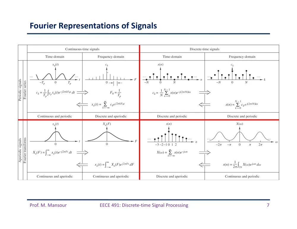
Frequency‐Domain and Time‐Domain Signal Properties
Continuous‐time
–
Fourier Series for periodic signals
–
Fourier Transform for aperiodic signals
Discrete‐time
–
Fourier Series for periodic signals
–
Fourier Transform for aperiodic signals
Prof. M. Mansour
EECE 491: Discrete‐time Signal Processing
6
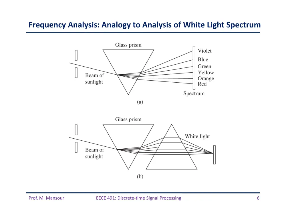
Frequency Analysis: Analogy to Analysis of White Light Spectrum
Prof. M. Mansour
EECE 491: Discrete‐time Signal Processing
7
Fourier Representations of Signals
Prof. M. Mansour
EECE 491: Discrete‐time Signal Processing
8
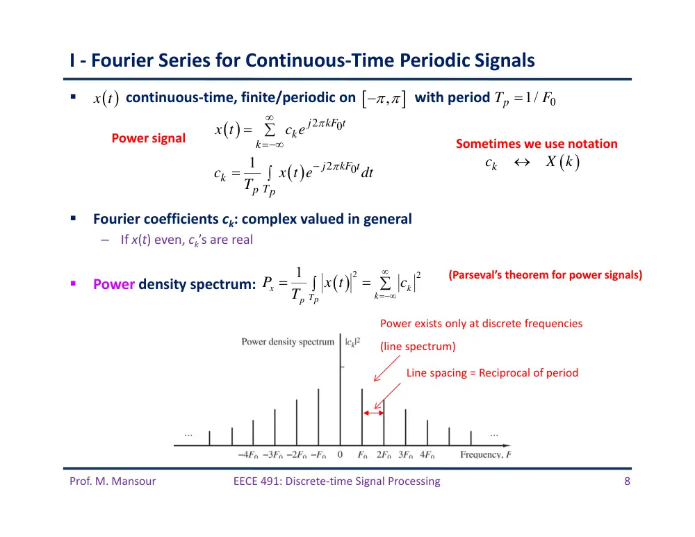
I ‐ Fourier Series for Continuous‐Time Periodic Signals
continuous‐time, finite/periodic on
with period
Fourier coefficients ck: complex valued in general
–
If x(t) even, ck’s are real
Power density spectrum:
2
0
2
0
1
j
kF t
k
k
j
kF t
k
p T
p
x t
c e
c
x t e
dt
T
2
2
1
x
k
k
p Tp
P
x t
c
T
Power exists only at discrete frequencies
(line spectrum)
Line spacing = Reciprocal of period
Power signal
(Parseval’s theorem for power signals)
kc
X k
Sometimes we use notation
x t
,
0
1/
Tp
F
Prof. M. Mansour
EECE 491: Discrete‐time Signal Processing
9
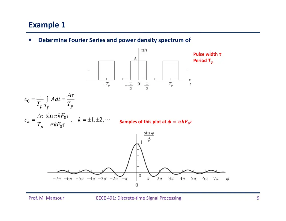
Example 1
Determine Fourier Series and power density spectrum of
0
0
0
1
sin
,
1, 2,
p T
p
p
k
p
A
c
Adt
T
T
kF
A
c
k
T
kF
Pulse width �
Period ��
Samples of this plot at � � �����
Prof. M. Mansour
EECE 491: Discrete‐time Signal Processing
10
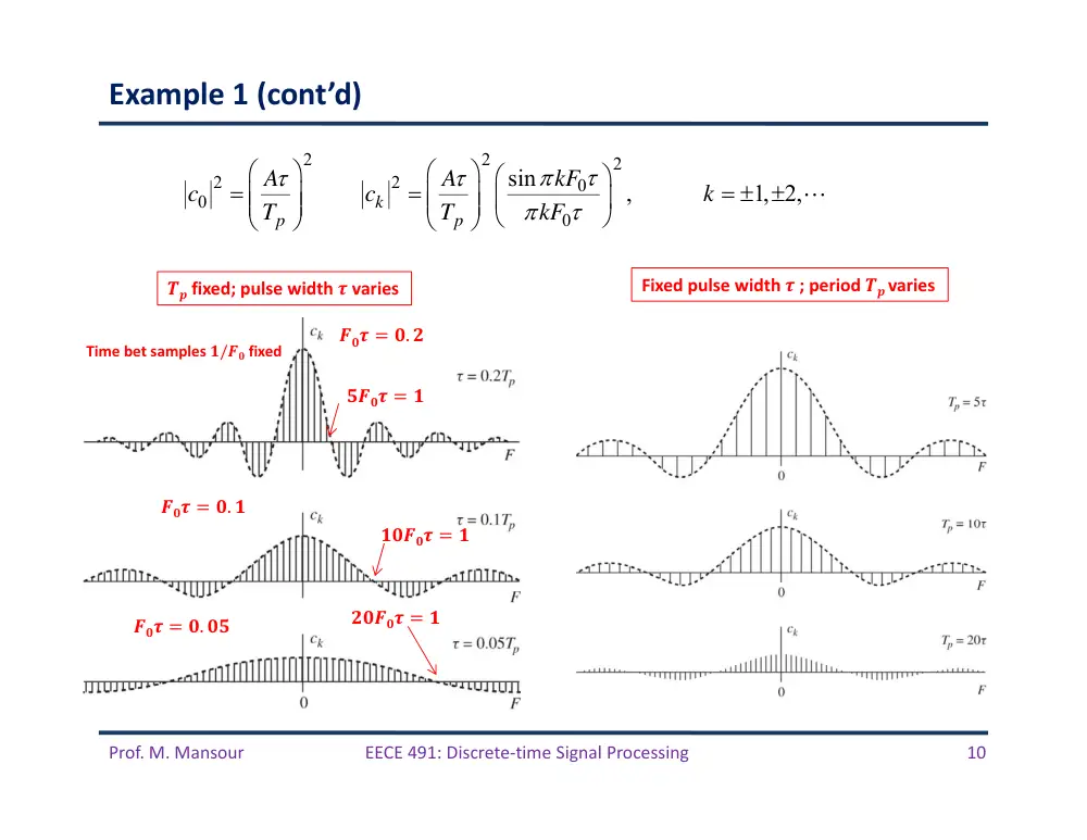
Example 1 (cont’d)
2
2
2
2
2
0
0
0
sin
,
1, 2,
k
p
p
kF
A
A
c
c
k
T
T
kF
�� fixed; pulse width � varies
Fixed pulse width � ; period �� varies
��� � �. �
���� � �
��� � �. �
����� � �
��� � �. ��
����� � �
Time bet samples �/�� fixed
Prof. M. Mansour
EECE 491: Discrete‐time Signal Processing
11
II ‐ Fourier Transform for Continuous Time Aperiodic Signals
x(t): continuous‐time, aperiodic with finite duration on [‐Tp/2, +Tp/2]
Energy:
2
2
j
Ft
j
Ft
x t
X F e
dF
X F
x t e
dt
x t
X F
2
1
2
j t
j t
F
x t
X
e
d
X
x t e
dt
Energy signal
2
2
Ex
x t
dt
X F
dF
Parseval’s theorem for aperiodic
finite energy signals
2
Sxx
X F
Energy density spectrum
(spectrum)
complex
Prof. M. Mansour
EECE 491: Discrete‐time Signal Processing
12
Example 2
Rectangular pulse
/2
2
/2
sin
j
Ft
X F
A
e
dt
F
A
F
2
Main lobe where most of the energy is
Prof. M. Mansour
EECE 491: Discrete‐time Signal Processing
13
Example 2 (cont’d)
Prof. M. Mansour
EECE 491: Discrete‐time Signal Processing
14
III ‐ Fourier Series for Discrete‐Time Periodic Signals
CT signal: periodic with period Tp
–
Frequency range extends from ‐ to . Can have infinite number of frequency
components
DT signal: periodic with period N
–
Frequency range is ‐ to . Can have at most N frequency components separated by
radians or f = 1/N cycles
Spectrum of a periodic signal x(n) with period N is a periodic sequence as well
with a period N.
Power density spectrum:
1
2
/
0
1
2
/
0
1
N
j
kn N
k
k
N
j
kn N
k
n
x n
c e
c
x n e
N
periodic
k N
k
c
c
kc
X k
Sometimes we use notation
1
1
2
2
0
0
1 N
N
x
k
n
k
P
x n
c
N
2
/ N
Prof. M. Mansour
EECE 491: Discrete‐time Signal Processing
15
Example 3
cos 2
x n
n
Spectrum of
Real since x(n) even
Spectrum of
with period 4
x n 1,1,0,0
Prof. M. Mansour
EECE 491: Discrete‐time Signal Processing
16
Example 4
Find spectrum of the DT periodic square wave below
1
2
/
0
1 /
1
,
0,1,
,
1
0,
,
sin
/
otherwise
sin
/
L
j
kn N
k
n
j k L
N
c
Ae
k
N
N
AL
k
N
N
kL N
A e
N
k
N
Prof. M. Mansour
EECE 491: Discrete‐time Signal Processing
17
IV‐ Fourier Transform of DT Aperiodic Signals (DTFT)
Frequency range of is ‐ to .
is periodic
Energy:
2
1
2
j n
j n
n
x n
X
e
d
X
x n e
2
2
1
2
x
n
E
x n
X
d
Parseval’s theorem for aperiodic
finite energy signals
2
Sxx
X
Energy density spectrum
j
X e
Sometimes written as
j
X e
j
X e
Prof. M. Mansour
EECE 491: Discrete‐time Signal Processing
18
Convergence of the Fourier Transform (DTFT)
Define the periodic version
converges uniformly to as
–
That is for every w,
Uniform convergence is guaranteed if x(n) is absolutely summable:
However, some sequences are not absolutely summable, but are square
summable, i.e., they have finite energy (weaker condition)
j n
n
X
x n e
N
j n
N
n
N
X
x n e
if
n
j n
n
n
x n
X
x n e
x n
2
x
n
E
x n
XN
X
N
as
XN
X
N
Prof. M. Mansour
EECE 491: Discrete‐time Signal Processing
19
Example 5
Consider important class of finite‐energy signals:
Its inverse FT is
1
0
c
c
X
0
sin
0
c
c
c
n
x n
n
n
n
Prof. M. Mansour
EECE 491: Discrete‐time Signal Processing
20
Example 5 (cont’d)
Now determine the DTFT of
x(n) is not absolutely summable but is square summable (i.e. has finite energy).
Hence the sequence below converges in the mean‐square sense
To illustrate this, define the finite sum
0
sin
0
c
c
c
n
x n
n
n
n
sin
j n
j n
c
n
n
n
x n e
e
n
sin
N
j n
c
N
n
N
n
X
e
n
Prof. M. Mansour
EECE 491: Discrete‐time Signal Processing
21
Example 5 (cont’d): Gibbs Phenomenon
sin
N
j n
c
N
n
N
n
X
e
n
oscillatory overshoot at
As � increases, oscillations become more rapid
But size of ripple stays the same
c
Prof. M. Mansour
EECE 491: Discrete‐time Signal Processing
22
Summary
1. CT signals have aperiodic spectra
–
Lack of periodicity due to the fact that the complex exponential is a function of a
continuous variable t, and hence not periodic in F.
–
Frequency range extends from �∞ to ∞
2. DT signals have periodic spectra: Both the Fourier series and the Fourier
transform are periodic with period
3. Periodic signals have discrete spectra
–
They are described by means of Fourier series
–
Coefficients provide “lines” that constitute the spectrum
–
Line spacing
4. Aperiodic energy signals have continuous spectra
–
Follows from the fact that is a function of and is a function of ,
which are continuous in the variables F and .
•
Periodicity with “period” � in one domain implies discretization with
“spacing” 1/� in the other domain
•
The converse is also true
j2
Ft
e
2
1/
or
1/
p
f
N
F
T
X F
j2
Ft
e
X
j n
e
Prof. M. Mansour
EECE 491: Discrete‐time Signal Processing
23
Symmetry Properties of DTFT
real
x n
Prof. M. Mansour
EECE 491: Discrete‐time Signal Processing
24
Symmetry Properties of DTFT
Prof. M. Mansour
EECE 491: Discrete‐time Signal Processing
25
Example 6
Draw the
for the Fourier transform
1
,
1
j
X
ae
,
,
,
R
I
X
X
X
X
Prof. M. Mansour
EECE 491: Discrete‐time Signal Processing
26
Example 7
Determine the DTFT of
Since x(‐n) = x(n) then X(w) is real.
Obtain
0
elsewhere
A
M
n
M
x n
1
sin
2
sin
/ 2
M
X
A
Prof. M. Mansour
EECE 491: Discrete‐time Signal Processing
27
Important Fourier Transform Theorems
Prof. M. Mansour
EECE 491: Discrete‐time Signal Processing
28
The Concept of Bandwidth
Prof. M. Mansour
EECE 491: Discrete‐time Signal Processing
29
Examples of Bandlimited Signals
Prof. M. Mansour
EECE 491: Discrete‐time Signal Processing
30
Outline
Part II: Frequency analysis of LTI systems
Prof. M. Mansour
EECE 491: Discrete‐time Signal Processing
31
Response of LTI Systems to Complex Exponentials
LTI system:
Excite with an exponential of amplitude A and frequency w:
Response:
The function
exists if system is BIBO stable (h(n) absolutely summable):
Hence the response is
–
Same frequency, but amplitude multiplied by H(w)
k
y n
h k x n
k
j n,
x n
Ae
n
j k
j n
k
y n
A
h k e
e
j k
k
H
h k e
k
h k
j n
y n
AH
e
H
Prof. M. Mansour
EECE 491: Discrete‐time Signal Processing
32
Example 1
Find response of system h(n) to x(n):
Solution:
Input has frequency
1
2
n
h n
u n
j n/2,
x n
Ae
n
1
1
1
2
j k
j
k
H
h k e
e
26.6
1
2
1
2
5
1
2
j
H
e
j
26.6
/2
/2 26.6
2
5
2
,
5
j
j n
j
n
y n
A
e
e
Ae
n
/ 2
Prof. M. Mansour
EECE 491: Discrete‐time Signal Processing
33
Example 2
Determine H(w) for the moving average filter:
Solution:
1
1
1
3
y n
x n
x n
x n
1 1 1
, ,
3 3 3
h n
1
1
1
1
2cos
3
3
j
j
H
e
e
1 1
2cos
3
H
0,
0
2
/ 3
,
2
/ 3
even
odd
Prof. M. Mansour
EECE 491: Discrete‐time Signal Processing
34
Response to other Sinusoids
1
1
j
j n
j n
x
n
Ae
y
n
A H
e
e
2
2
j
j n
j n
j
j n
x
n
Ae
y
n
A H
e
e
A H
e
e
1
2
1
2
1
cos
2
1
cos
2
x n
x
n
x
n
A
n
y n
y
n
y
n
A H
n
1
2
1
2
1
sin
2
1
sin
2
x n
x
n
x
n
A
n
j
y n
y
n
y
n
A H
n
Prof. M. Mansour
EECE 491: Discrete‐time Signal Processing
35
Example 3
Find response to this input:
Solution:
10
5sin
20cos
,
2
x n
n
n
n
1
1
1
2
j
H
e
1
@
0:
0
2
1
1
2
H
26.6
2
@
2 :
2
5
j
H
e
2
@
:
3
H
10
40
20
sin
26.6
cos
,
2
3
5
y n
n
n
n
Prof. M. Mansour
EECE 491: Discrete‐time Signal Processing
36
Response to Aperiodic Signals
From convolution theorem:
Output of an LTI system cannot contain frequency components that are not
contained in the input signal
–
An LTI system can only cause magnitude and phase distortion
The output response can be obtained as
Also
Y
H
X
2
1
2
j n
y n
Y
e
d
2
2
2
2
yy
xx
Y
H
X
S
H
S
2
2
2
1
2
1
2
y
yy
xx
E
S
d
H
S
d
Energy density spectrum
Prof. M. Mansour
EECE 491: Discrete‐time Signal Processing
37
Example 4
Find response of system h(n) to x(n):
Solution:
1
2
n
h n
u n
1
4
n
x n
u n
1
1
1
2
j k
j
k
H
h k e
e
1
1
1
1
1
2
4
j
j
Y
H
X
e
e
1
1
1
4
j
X
e
2
1
5
17
1
cos
cos
4
16
2
yy
xx
S
H
S
Prof. M. Mansour
EECE 491: Discrete‐time Signal Processing
38
Frequency Response of LTI Systems
For rational transfer functions, we have:
j n
z e j
n
H
H z
h n e
A z
H z
B z
0
1
0
1
1
1
1
1
M
M
j
j k
k
k
k
k
N
N
j k
j
k
k
k
k
z e
b e
H
b
a e
p e
1
0
1
0
1
1
1
1
1
1
M
M
k
k
k
k
k
N
N
k
k
k
k
k
z z
b z
H z
b
a z
p z
B
H
A
* *
*
*
*
1
1
0
0
* *
*
1
1
1
1
1/
1
1
M
M
k
k
k
k
N
N
k
k
k
k
z z
z z
H
z
b
b
p z
p z
*
*
*
*
*
1
1
0
0
*
*
1
1
1/
1
1
1
1
z e j
M
M
j
j
k
k
k
k
N
N
j
j
k
k
k
k
H
H
z
z e
z e
b
b
p e
p e
coefficients
zeros
poles
Prof. M. Mansour
EECE 491: Discrete‐time Signal Processing
39
Frequency Response of LTI Systems
For real coefficients ak’s and bk’s (i.e., when h(n) is real):
–
Zeros (zk’s ) and poles (pk’s ) are either real or occur in complex conjugate pairs
Therefore, we have
This implies
We know that
2
*
H
H
H
*
*
1
1/
H
z
H z
and
H*
H
2
*
1
z e j
H
H
H
H
H
H z H z
1
hh
hh
r
l
h l
h
l
R
z
H z H z
2
Fourier Transform
hh
H
r
l
Prof. M. Mansour
EECE 491: Discrete‐time Signal Processing
40
Example 5
Determine
for the system:
Solution:
–
ROC includes unit circle, hence
exists
0.1
1
0.2
2
1
y n
y n
y n
x n
x n
1
1
2
1
,
ROC:
0.5
1
0.1
0.2
z
H z
z
z
z
1
1
1
2
2
1
1
2
2
1
1
1
0.1
0.2
1
0.1
0.2
2
1.05
0.08
0.2
z
z
H z H z
z
z
z
z
z
z
z
z
z
z
2
2
2 1
cos
1.45
0.16cos
0.8cos
H
2
H
H
Prof. M. Mansour
EECE 491: Discrete‐time Signal Processing
41
Computation of the Frequency Response Function
Express in polar form:
1
1
0
0
1
1
1
1
M
M
j
j
k
k
j
N M
k
k
N
N
j
j
k
k
k
k
z e
e
z
H
b
b e
p e
e
p
j
j
k
k
k
j
j
k
k
k
e
z
V
e
e
p
U
e
Evaluate H(w) at w
Evaluate H(z) at point L
,
j
k
e
p
CL
CA
CL
CA
AL
,
j
k
e
z
CL
CB
CL
CB
BL
j
j
k
k
k
j
j
k
k
k
e
p
U
e
e
z
V
e
AL
BL
N
M
Prof. M. Mansour
EECE 491: Discrete‐time Signal Processing
42
Computation of the Frequency Response Function
Phase interpretation:
Prof. M. Mansour
EECE 491: Discrete‐time Signal Processing
43
Geometric Interpretation of Poles and Zeros
Assume a zero zk and a pole pk are on the unit circle
Presence of a zero close to unit circle causes at frequencies that correspond to
points on unit circle close to that point, to be small
Poles have opposite effect
Placing a pole close to a zero cancels effect of zero, and vice versa
j
j
k
k
k
j
j
k
k
k
e
z
V
e
e
p
U
e
,
and consequently
become zero
k
k
At
z V
H
,
becomes 0 and consequently
becomes
k
k
At
p U
H
H
Prof. M. Mansour
EECE 491: Discrete‐time Signal Processing
44
Example 6
Find the frequency response of:
Solution: H has
–
Zero at � � 0
–
Pole at � � 0.8
1
1
0.8
1
0.8
z
H z
z
z
0.8
j
j
e
H
e
1
1
1.64 1.6cos
sin
tan
cos
0.8
H
Frequency
closest to pole
Prof. M. Mansour
EECE 491: Discrete‐time Signal Processing
45
Part III: LTI Systems as Frequency Selective Filters
Prof. M. Mansour
EECE 491: Discrete‐time Signal Processing
46
Ideal Frequency Selective Discrete‐Time Filters
Magnitude responses
What about phase?
Y
H
X
Prof. M. Mansour
EECE 491: Discrete‐time Signal Processing
47
Phase Response of Ideal Filters
An ideal filter has linear phase response. Why?
Assume a signal is passed through a filter with frequency response:
In general, linear phase
The derivative of is called group delay:
–
Time delay that a signal component at frequency w undergoes as it passes through filter
0
1
2
0
elsewhere
Ce j n
H
C, n0 constants
0
1
2
j n ,
Y
H
X
CX
e
0
y n
Cx n
n
Linear phase translates into delay
This is tolerable and not considered distortion
Phase: –wn0
g
d
d
n0