EECE 491 Lecture 4, Spring 2016

Prof. M. Mansour EECE 491: Discrete‐time Signal Processing 1 EECE 491: Discrete‐time Signal Processing Mohammad M. Mansour Dept. of Electrical and Compute Engineering American University of Beirut Lecture 4: Z‐Transform Prof. M. Mansour EECE 491: Discrete‐time Signal Processing 2 Announcements  Reading – Chapter 3, Proakis Prof. M. Mansour EECE 491: Discrete‐time Signal Processing 3 The Z‐Transform  Used for: – Analysis of LTI systems – Solving difference equations – Determining system stability – Finding frequency response of stable systems Prof. M. Mansour EECE 491: Discrete‐time Signal Processing 4 Eigen Functions of LTI System  Consider an LTI system with an impulse response h[n]:  Let  Output is the same pure frequency, scaled and phase‐shifted!  Therefore, is an Eigen‐function of an LTI system           0 0 0 0 0 j n k k j k j n k j n j y n h k e h k e e H e e                                 DTFT H e j h n     j 0 n x n e   j 0 e  n Prof. M. 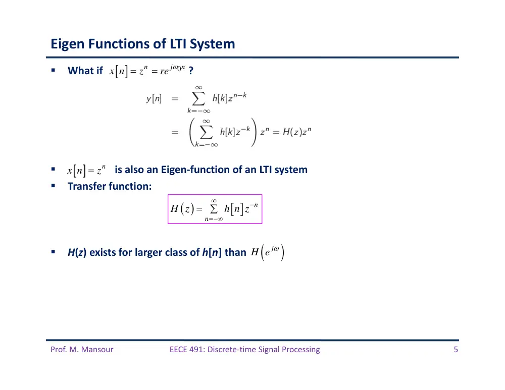Mansour EECE 491: Discrete‐time Signal Processing 5 Eigen Functions of LTI System  What if ?  is also an Eigen‐function of an LTI system  Transfer function:  H(z) exists for larger class of h[n] than     n n H z h n z        j 0 n n x n z re      n x n z   j  H e  Prof. M. 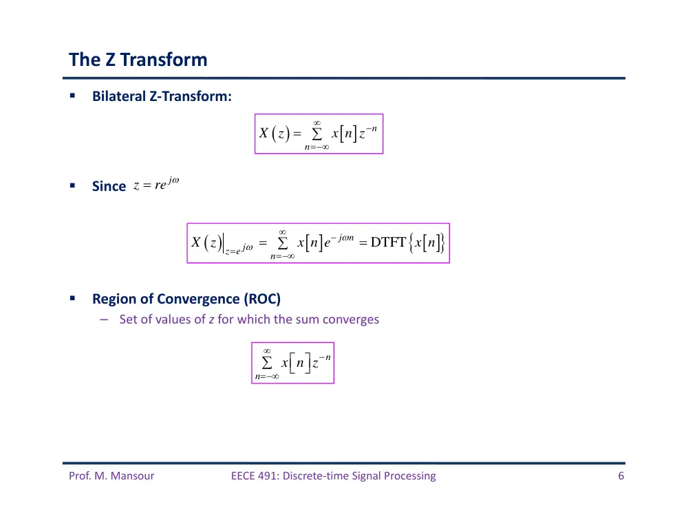Mansour EECE 491: Discrete‐time Signal Processing 6 The Z Transform  Bilateral Z‐Transform:  Since  Region of Convergence (ROC) – Set of values of z for which the sum converges     n n X z x n z              DTFT j n z e j n X z x n e x n          j z re   x n  zn n   Prof. M. 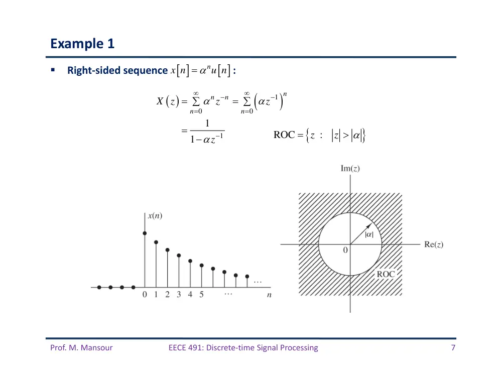Mansour EECE 491: Discrete‐time Signal Processing 7 Example 1  Right‐sided sequence :     1 0 0 1 1 1 n n n n n X z z z z                   ROC z : z      n   x n   u n Prof. M. 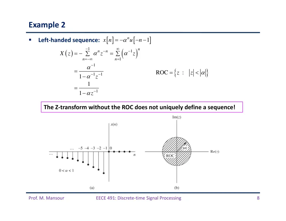Mansour EECE 491: Discrete‐time Signal Processing 8 Example 2  Left‐handed sequence:     1 1 1 1 1 1 1 1 1 1 n n n n n X z z z z z                           ROC z : z    The Z‐transform without the ROC does not uniquely define a sequence!    1 n x n u n     Prof. M. 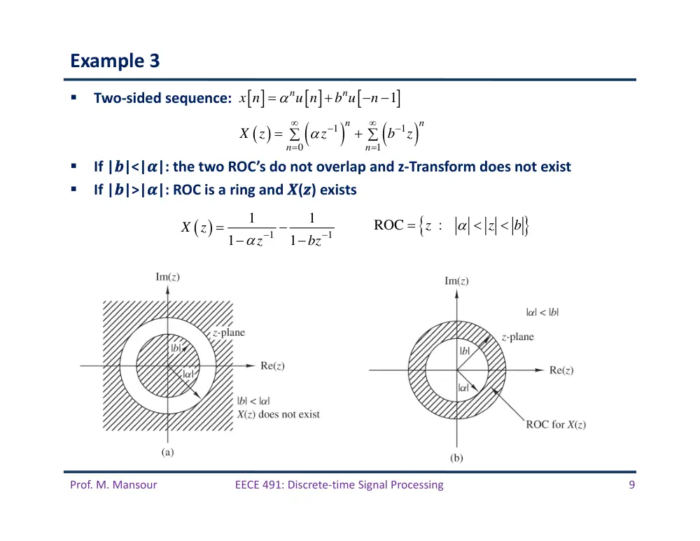Mansour EECE 491: Discrete‐time Signal Processing 9 Example 3  Two‐sided sequence:  If |�|<|�|: the two ROC’s do not overlap and z‐Transform does not exist  If |�|>|�|: ROC is a ring and �(�) exists       1 1 0 1 n n n n X z z b z              1 1 1 1 1 1 X z z bz          ROC z : z b          1 n n x n u n b u n      Prof. M. 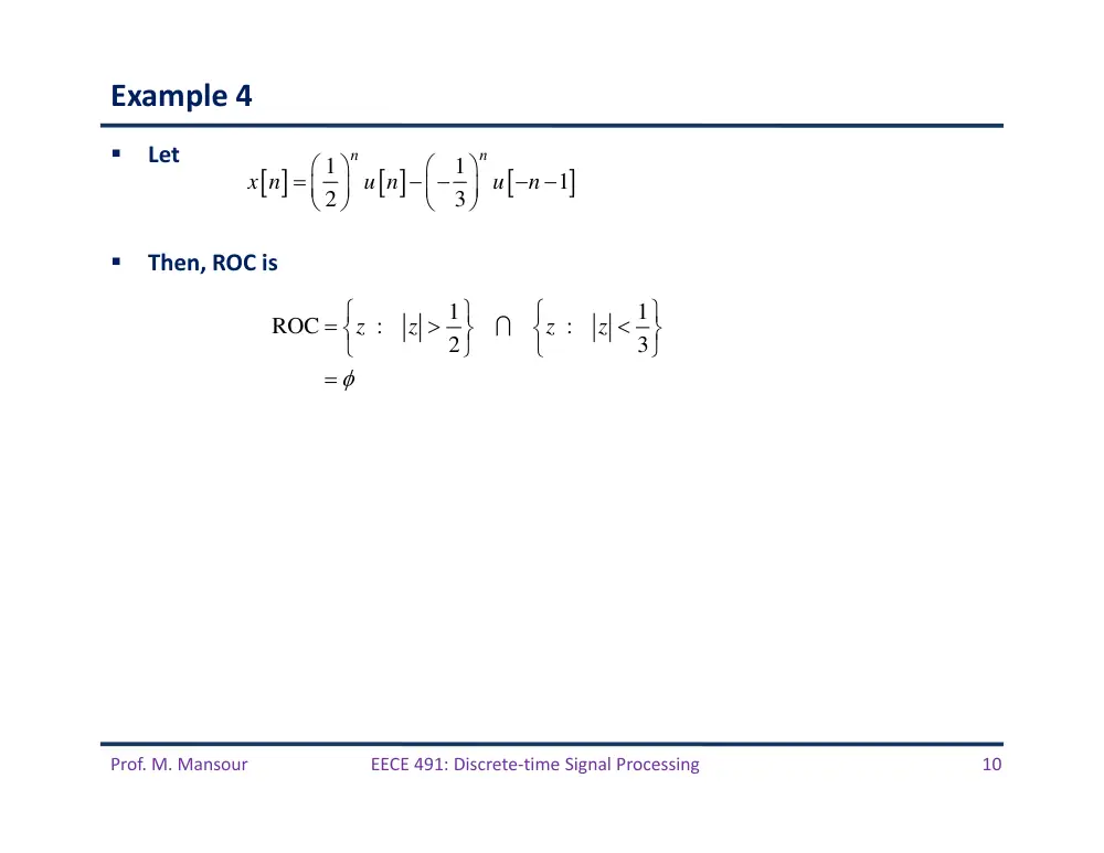Mansour EECE 491: Discrete‐time Signal Processing 10 Example 4  Let  Then, ROC is 1 1 ROC : : 2 3 z z z z                         1 1 1 2 3 n n x n u n u n                  Prof. M. Mansour EECE 491: Discrete‐time Signal Processing 11 Example 5  Let     ROC : : z z a z z a         , 0 n x n a a   Prof. M. Mansour EECE 491: Discrete‐time Signal Processing 12 Example 6  Finite sequence:   ROC : 0 z z     1 0 1 2 1 1 1 Finite, always converges 1 zero cancels the pole 1 = 1 M n n n M M k M j M k X z a z a z az ae z                              1 n x n a u n u n M     Prof. M. Mansour EECE 491: Discrete‐time Signal Processing 13 Properties of the ROC  P1: A ring or a disk in the Z‐plane, centered at the origin  P2: DTFT converges iff ROC includes the unit circle  P3: ROC cannot contain poles  P4: For finite duration sequences, ROC is the entire Z‐plane, except possibly z = 0 or z = 1 Prof. M. Mansour EECE 491: Discrete‐time Signal Processing 14 Properties of the ROC  P5: For right‐sided sequences (x[n] = 0 for all n < N1, for some N1) ROC extends outward from the outer‐most pole to infinity.  P6: For left‐sided sequences (x[n] = 0 for all n > N2, for some N2 ) ROC extends inwards from the inner‐most pole to zero.  P7: For two‐sided sequences, ROC is a ring – Inner‐bound: Pole with largest magnitude that contributes for n > 0 – Outer‐bound: Pole with smallest magnitude that contributes for n < 0 Prof. M. Mansour EECE 491: Discrete‐time Signal Processing 15 Characteristic Families of Signals with their ROCs finite infinite Prof. M. Mansour EECE 491: Discrete‐time Signal Processing 16 Several Properties of the Z Transform Prof. M. Mansour EECE 491: Discrete‐time Signal Processing 17 Some Common z‐Transform Pairs Prof. M. Mansour EECE 491: Discrete‐time Signal Processing 18 Inversion of the Z‐Transform  In general, we can invert by contour integration within the ROC:  Ways to avoid it: – Inspection (known transforms) – Properties of the Z‐transform – Power series expansion – Partial fraction expansion – Residue theorem  Most useful is the inverse of rational polynomials       B z X z  A z Prof. M. Mansour EECE 491: Discrete‐time Signal Processing 19 Causal LTI Systems  Described by linear constant‐coefficient difference equations:       1 0 N M k k k k y n a y n k b x n k                0 0 1 M k k k M k k k b z Y z H z X z a z          Prof. M. Mansour EECE 491: Discrete‐time Signal Processing 20 Inversion of the Z‐Transform Prof. M. Mansour EECE 491: Discrete‐time Signal Processing 21 Inversion of the Z‐Transform Prof. M. Mansour EECE 491: Discrete‐time Signal Processing 22 Inversion of the Z‐Transform  Example: Partial Fraction Expansion Prof. M. Mansour EECE 491: Discrete‐time Signal Processing 23 Inversion of the Z‐Transform Prof. M. Mansour EECE 491: Discrete‐time Signal Processing 24 Inversion of the Z‐Transform Prof. M. Mansour EECE 491: Discrete‐time Signal Processing 25 Inversion of the Z‐Transform Prof. M. Mansour EECE 491: Discrete‐time Signal Processing 26 Example 7 Prof. M. Mansour EECE 491: Discrete‐time Signal Processing 27 Time‐Domain Behavior of a Single Real Pole Causal Signal Prof. M. Mansour EECE 491: Discrete‐time Signal Processing 28 Time‐Domain Behavior of a Double Real Pole Causal Signal Prof. M. Mansour EECE 491: Discrete‐time Signal Processing 29 Time‐Domain Behavior of a Pair of Complex‐Conjugate Poles Prof. M. Mansour EECE 491: Discrete‐time Signal Processing 30 Stability and Causality of the z‐Transform  Causal: ROC extends from outermost pole  BIBO stable:  Consider the unit circle z = ejw. In this case we have . Then  Hence, BIBO stability  ROC of H(z) includes the unit circle zero pole 1 n j n z e     