EECE 491 Lecture 2, Fall 2015

Prof. M. Mansour EECE 491: Discrete‐time Signal Processing 1 EECE 491: Discrete‐time Signal Processing Mohammad M. Mansour Dept. of Electrical and Compute Engineering American University of Beirut Lecture 2: Review of Signals, Systems, and Signal Processing Prof. M. Mansour EECE 491: Discrete‐time Signal Processing 2 Announcements  Reading – Chapter 1, Proakis Prof. M. Mansour EECE 491: Discrete‐time Signal Processing 3 Outline  Signals and signal types – Continuous‐time vs. discrete‐time frequency – Harmonically‐related complex exponentials  SP systems  Sampling  A/D and D/A  Quantization – SQNR Prof. M. 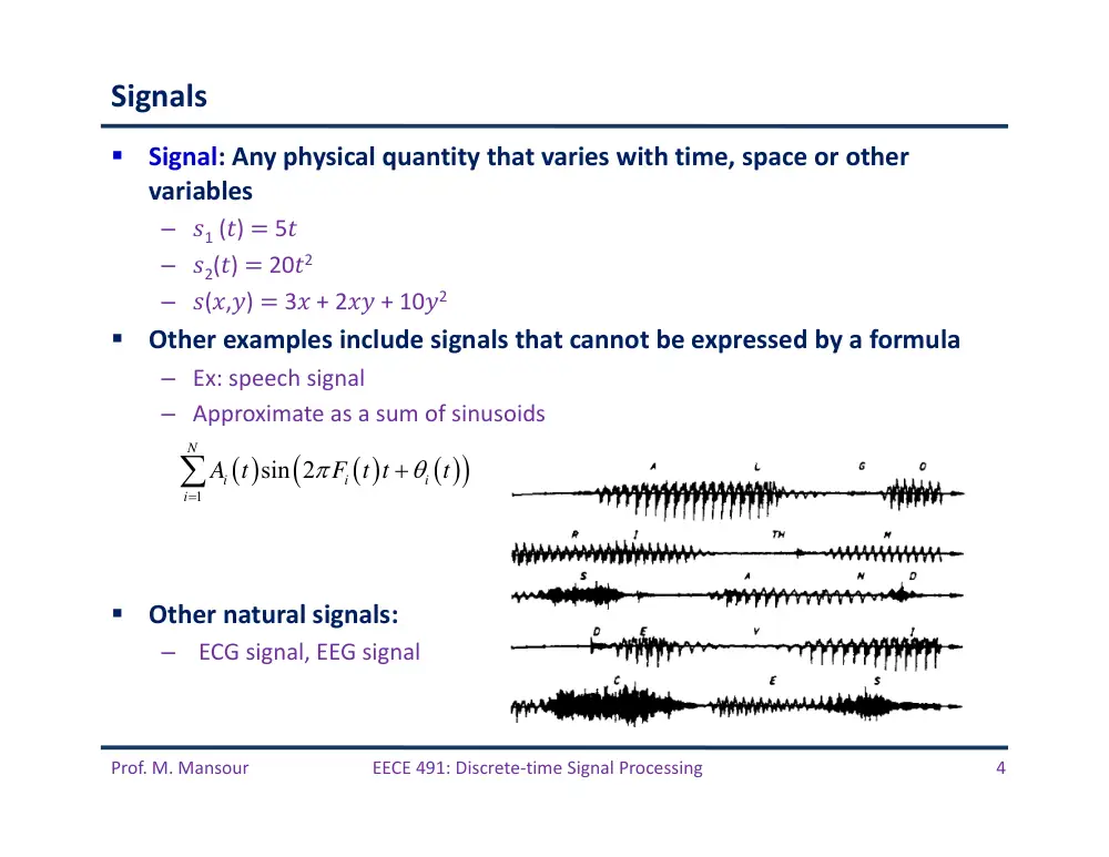Mansour EECE 491: Discrete‐time Signal Processing 4 Signals  Signal: Any physical quantity that varies with time, space or other variables – �1 (�) � 5� – �2(�) � 20�2 – �(�,�) � 3� + 2�� + 10�2  Other examples include signals that cannot be expressed by a formula – Ex: speech signal – Approximate as a sum of sinusoids  Other natural signals: – ECG signal, EEG signal         1 sin 2 N i i i i A t F t t t      Prof. M. 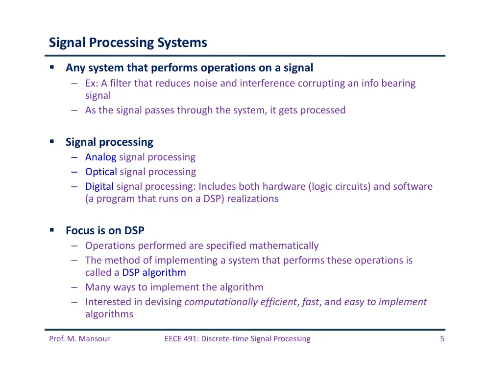Mansour EECE 491: Discrete‐time Signal Processing 5 Signal Processing Systems  Any system that performs operations on a signal – Ex: A filter that reduces noise and interference corrupting an info bearing signal – As the signal passes through the system, it gets processed  Signal processing – Analog signal processing – Optical signal processing – Digital signal processing: Includes both hardware (logic circuits) and software (a program that runs on a DSP) realizations  Focus is on DSP – Operations performed are specified mathematically – The method of implementing a system that performs these operations is called a DSP algorithm – Many ways to implement the algorithm – Interested in devising computationally efficient, fast, and easy to implement algorithms Prof. M. 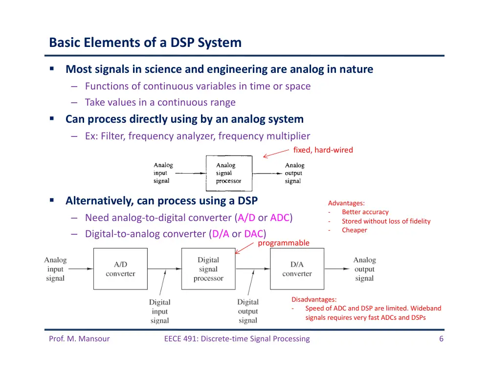Mansour EECE 491: Discrete‐time Signal Processing 6 Basic Elements of a DSP System  Most signals in science and engineering are analog in nature – Functions of continuous variables in time or space – Take values in a continuous range  Can process directly using by an analog system – Ex: Filter, frequency analyzer, frequency multiplier  Alternatively, can process using a DSP – Need analog‐to‐digital converter (A/D or ADC) – Digital‐to‐analog converter (D/A or DAC) fixed, hard‐wired programmable Advantages: ‐ Better accuracy ‐ Stored without loss of fidelity ‐ Cheaper Disadvantages: ‐ Speed of ADC and DSP are limited. Wideband signals requires very fast ADCs and DSPs Prof. M. 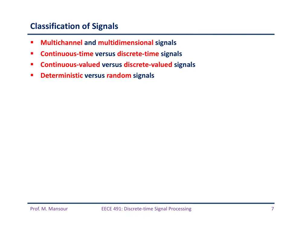Mansour EECE 491: Discrete‐time Signal Processing 7 Classification of Signals  Multichannel and multidimensional signals  Continuous‐time versus discrete‐time signals  Continuous‐valued versus discrete‐valued signals  Deterministic versus random signals Prof. M. 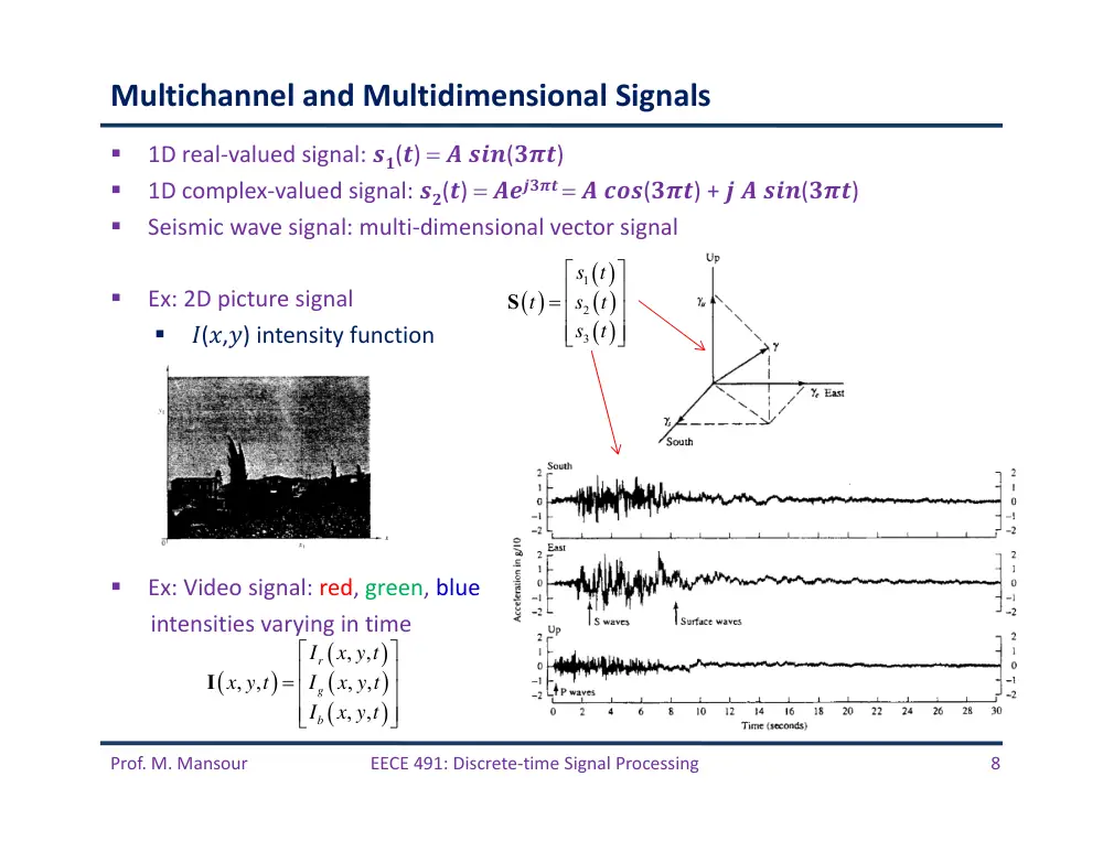Mansour EECE 491: Discrete‐time Signal Processing 8  1D real‐valued signal: ��(�)  � ���(���)  1D complex‐valued signal: ��(�)  ������  � ���(���) + � � ���(���)  Seismic wave signal: multi‐dimensional vector signal  Ex: 2D picture signal  �(�,�) intensity function  Ex: Video signal: red, green, blue intensities varying in time Multichannel and Multidimensional Signals         1 2 3 s t t s t s t            S         , , , , , , , , r g b I x y t x y t I x y t I x y t            I Prof. M. 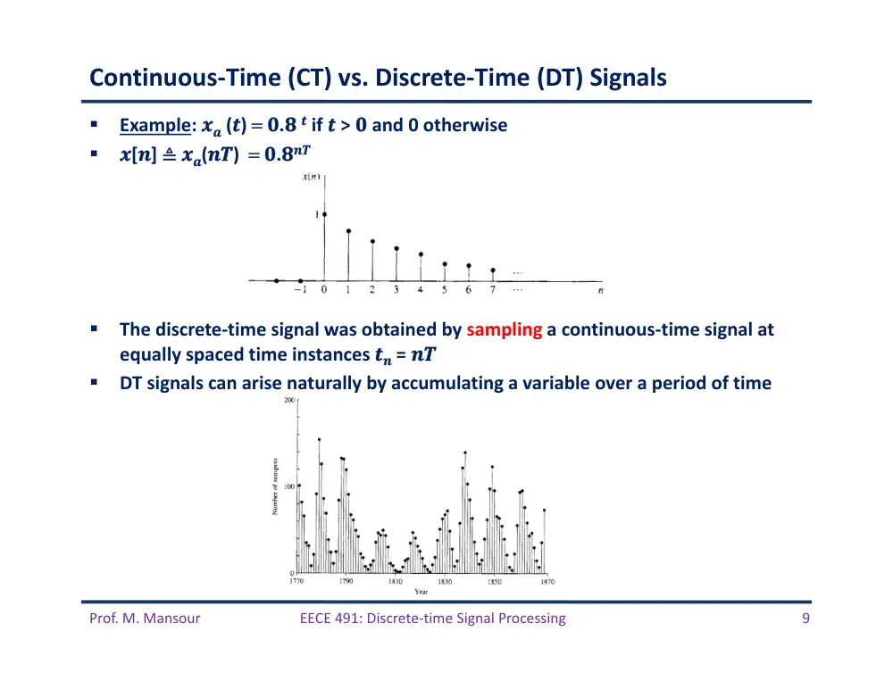Mansour EECE 491: Discrete‐time Signal Processing 9 Continuous‐Time (CT) vs. Discrete‐Time (DT) Signals  Example: �� (�)  �.� � if � > � and 0 otherwise  �[�] ≜ ��(��)   �.���  The discrete‐time signal was obtained by sampling a continuous‐time signal at equally spaced time instances �� = ��  DT signals can arise naturally by accumulating a variable over a period of time Prof. M. 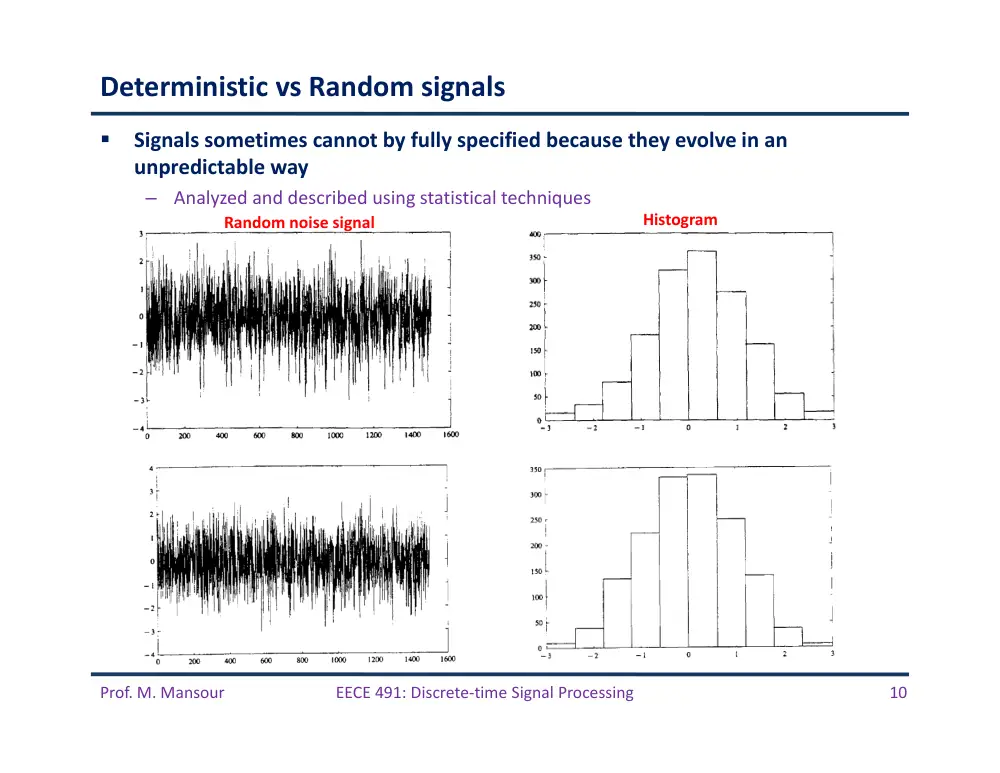Mansour EECE 491: Discrete‐time Signal Processing 10 Deterministic vs Random signals  Signals sometimes cannot by fully specified because they evolve in an unpredictable way – Analyzed and described using statistical techniques Random noise signal Histogram Prof. M. Mansour EECE 491: Discrete‐time Signal Processing 11 Continuous‐Valued vs Discrete‐Valued Signals  Values of a CT and DT signals can continuous or discrete  Discrete valued DT signals are called digital signals  Digital signals are obtained by quantizing a sampled CT signal Prof. M. Mansour EECE 491: Discrete‐time Signal Processing 12 Frequency of a CT Signal  �� (�) = ����(��+�),     −∞ < � < ∞ – A: Amplitude – �: Frequency in rad/sec; �=���,   � is frequency in cycles/sec (Hz) – �: Phase in radians  Properties of analog sinusoidal signals – For any fixed �, ��(�) is periodic with �� = 1/F being its fundamental period – CT sinusoidal signals with different frequencies are themselves different – Increasing F results in an increase in the rate of oscillation  These properties apply to class of complex‐exponential signals as well – �� (�) = ���(��+�) = ����(��+�) + �����(��+�)  For mathematical convenience we use negative frequencies – ���(��+�) = �/� ��(��+�)  + �/� ��(��−�) – Phasor representation Prof. M. Mansour EECE 491: Discrete‐time Signal Processing 13 Frequency of a DT Signal  – A: Amplitude – �=���: Frequency in rad/sample;   � is frequency in cycles/sample (Hz) – �: Phase in radians 1. Properties of DT sinusoidal signals: A DT sinusoid is periodic with period N if f is rational. – Periodic: Smallest N that satisfies x[n+N] = x[n] for all n is called fundamental period – Ex: for a sinusoid with freq f0: – Ex: – Ex:       0 0 0 cos 2 cos 2 : 2 2 f N n f n k f N k                1 1 31/ 60 60 f N    2 2 30 / 60 2 f N          cos , a x n x nT n n           Prof. M. Mansour EECE 491: Discrete‐time Signal Processing 14 Properties of DT Sinusoidal Signals (cont’d) 2. DT sinusoids whose frequencies are integer multiples of �� are identical  Hence, all sinusoidal sequences �� (�)= ����(���+�), � = 0,1,…  are identical when �� = ��+ 2�k, where −� ≤ �� ≤ �  Any sequence resulting from a sinusoid with freq |�| > � is identical to a sequence obtained from a sinusoidal signal with|�| < �  Sinusoids with |�| > � are called aliases  Frequencies in the range −� ≤ � ≤ � or −1/2 ≤ � ≤ 1/2  are unique – Frequencies in the range |�| > � or |�| > 1/2 are aliases  Ex: for � ≤ �� ≤ 2�, consider two sinusoids with freqs ��=�� and �� = 2� −�� – ��[�] = ����(��� + �) – ��[�] = ����(���+�) = ����((��−��)�+�) = �1[�]       0 0 cos 2 cos n n          Prof. M. Mansour EECE 491: Discrete‐time Signal Processing 15 Properties of DT Sinusoidal Signals (cont’d) 3. The highest rate of oscillation is attained when � =± � or � = ±1/2 Prof. M. Mansour EECE 491: Discrete‐time Signal Processing 16 Harmonically‐Related Complex Exponentials (HRCEs)  Harmonically‐Related Complex Exponentials: Set of periodic complex exponentials with fundamental frequencies multiple of a single frequency  CT exponentials: – Fundamental period: 1/(��0) = ��/� – Fundamental freq: ��0 – Periodic signals with period ��/� and hence also with period ��. – F0 can take any value and all members of the set are distinct  Basic signals are a linear combination of HRCEs: – ��: arbitrary complex constants – ��(�) is periodic with fundamental period �� = 1/�0. – Representation is called Fourier series expansion of ��(�) and��’s are Fourier series coefficients. – ��(�) is called the kth harmonic   0 0 2 , 0, 1, 2, jk t j kF t ks t e e k             0 jk t a k k k k k x t c s t c e          Prof. M. Mansour EECE 491: Discrete‐time Signal Processing 17 Discrete‐Time Exponentials  A DT complex exponential is periodic if its relative frequency is a rational number, choose �0 = 1/�  Define the set of DT‐HRCEs as  Note that  Hence there are only N distinct DT‐HRCEs in the above set  All members have a common period of N samples  Choose any consecutive N complex exponentials to form the set of HRCEs – Most convenient choice:  Linear combination: – Periodic with period N – Called Fourier series expansion for a periodic DT signal, with Fourier coefficients {��} – ��[�] is called the kth harmonic   0 2 , 0, 1, 2, j kf n ks n e k               0 2 2 j kf n N j n k N k k s n e e s n s n          2 / , 0,1, , 1 j kn N ks n e k N          1 1 2 / 0 0 N N j kn N k k k k k x n c s n c e          Prof. M. Mansour EECE 491: Discrete‐time Signal Processing 18 Example  Assume you have stored in memory of a DSP one cycle of the sinusoid: – �[�] = sin(���/�+�) where � = ���/�, where � and � are integers – i.e., the samples x[0], x[1], …, x[N‐1] are stored in the processor’s memory  Q1: Determine how this table of values can be used to obtain values of harmonically related sinusoids having the same phase – That is find �2[�] = sin(���2/�+�), �3[�] = sin(���3/�+�), …, �k[�] = sin(���k/�+�)  Answer: Let ��[�]= ���(����/�+�) having frequency ��= �/� which is harmonically related to x[n]. – ��[n] = ���(����/�+�) = �[�� mod N] – Read off values from memory for every n to determine all xk[n] – Ex: Assume N = 10, and k = 2. The 10 values of the harmonic sequence x2[n] are: – Ex: Assume N = 10, and k = 3. The 10 values of the harmonic sequence x3[n] are: x2[0] = x[0] x2[1] = x[2] x2[2] = x[4] x2[3] = x[6] x2[4] = x[8] x2[5] = x[0] x2[6] = x[2] x2[7] = x[4] x2[8] = x[6] x2[9] = x[8] (two periods) x3[0] = x[0] x3[1] = x[3] x3[2] = x[6] x3[3] = x[9] x3[4] = x[2] x3[5] = x[5] x3[6] = x[8] x3[7] = x[1] x3[8] = x[4] x3[9] = x[7] (one period) Prof. M. Mansour EECE 491: Discrete‐time Signal Processing 19 Example (cont’d)  Q2: Determine how this table of values can be used to obtain sinusoids having the same frequency but different phase. – That is given – Determine  Answer: – The same applies for any other phase     sin 2 / , 2 / kx n nk N q N            sin 2 / , 2 / ky n nk N N                        sin 2 / 2 / sin 2 / 2 / sin 2 1 / 1 k k y n nk N k N nk N k N n k N x n                    2 / m N       Prof. M. Mansour EECE 491: Discrete‐time Signal Processing 20 A/D and D/A Conversion Prof. M. Mansour EECE 491: Discrete‐time Signal Processing 21 A/D and D/A Conversion  Three steps: – Sampling: Take samples of a CT signal at discrete time instances: �[�]=��(��), T is the sampling period, and � = 1/� is the sampling rate. • Uniform or periodic sampling – Quantization: Convert a DT continuous‐valued signal into a digital signal. • x�[�] = �(�[�]), where |�[�]−��[�]| is the quantization error – Coding: Each discrete value ��[�] is mapped to a b‐bit binary number Prof. M. Mansour EECE 491: Discrete‐time Signal Processing 22 Sampling of Analog Signals  �[�] = ��(��),  −∞ < � < ∞  Sampling rate: �� = 1/� (samples per sec, Hertz)  Relationship between t and n: � = �� = �/��  Hence there exists a relationship between frequency F (analog signal) and f (DT signal) Prof. M. Mansour EECE 491: Discrete‐time Signal Processing 23 Sampling of Analog Signals (cont’d)  ��(�) = ����(����+�), when sampled at ��= 1/� gives  CT: −∞ < � < ∞        −∞ < Ω < ∞  DT: −�/�<�<�/� −�<�<�  Therefore:  Hence: The frequency of a CT sinusoid when sampled at a rate �� = 1/� must fall in the range −��/� ≤ � ≤ ��/�  Map an infinite frequency range of a CT signal into a finite frequency range for the DT signal  ���� = ��/2       cos , a x n x nT n n                   cos 2 / cos 2 1 2 2 2 a s s s s x nT x n A nF F A nf F f F F f F T F F                       1 1 1 1 2 2 2 2 2 2 s s s F F F F F T T           Prof. M. Mansour EECE 491: Discrete‐time Signal Processing 24 Example  Consider two CT signals sampled at Fs = 40Hz – �1(�) = ���2�(10)� – �2(�) = ���2�(50)�  Corresponding DT signals are: – �1(�) = ���2�(10/40)� = cos(�/2 �) – �2(�) = ���2�(50/40)� = cos(5�/2 �) = cos(�/2 �) – Therefore �1(�) = �2(�)  The two DT signals are identical and hence they are indistinguishable  We say that the frequency 50Hz is an alias of the frequency F1 = 10Hz at the sampling rate of 40 samples/sec.  Also all frequencies �1 + 40�, � = 0, 1, 2, … are aliases as well Prof. M. Mansour EECE 491: Discrete‐time Signal Processing 25 Sampling of Analog Signals (cont’d) Two cases:  Case I: If , then f0 is in the range                      . The relationship between F0 and f0 is one to one, and it is possible to reconstruct ��(�) from �[�].  Case II: Otherwise, for sinusoids                                             with frequencies ��= �0 +���, � =±�, ±�,… If they are sampled at Fs, it is clear that Fk is outside the fundamental range. Hence the sampled signal in this case is sample @ ��= �/� sample @�� = �/�     0 cos 2 ax t A  F t        0 0 0 cos 2 , a s F x n A f n f F      0 2 2 s s F F F    0 1 1 2 2 f        cos 2 a k x t A  F t        cos 2 a k x t A  F t        0 0 0 cos 2 cos 2 cos 2 s s s F kF x n A n F F A F n A f n                          Prof. M. Mansour EECE 491: Discrete‐time Signal Processing 26 Sampling of Analog Signals (cont’d) �0 � � � Hz �1 � � � � Hz 0 k s F F kF   1 0 7 1 8 F  F    Prof. M. Mansour EECE 491: Discrete‐time Signal Processing 27 Example  Consider the analog signal ��(�) = ����(�����)  Q1: Determine the minimum sampling rate required to avoid aliasing.  A1: ��,��� = 2×� = 2×50 = 100��  Q2: Suppose ��(�) is sampled at ��= 200Hz. What is the resulting DT signal?  A2:  Q3: Suppose ��(�) is sampled at �� = ��Hz. What is the resulting DT signal?  A3:  Q4: What is the frequency 0 < � < ��/2 of an analog sinusoid that yields samples identical to those in Q3?  A4: For the sampling rate ��= 75 Hz, we have � =�×�� = 75�. The frequency of the DT signal in Q3 is � = 1/3. So the frequency of the CT signal is � = 25 Hz and the corresponding sinusoid is ��(�) = ����(����)   3cos 100 3cos 200 2 n n x n                   100 4 2 3cos 3cos 3cos 75 3 3 n n n x n                         Prof. M. Mansour EECE 491: Discrete‐time Signal Processing 28 The Sampling Theorem  Need to know the maximum frequency content of a signal to sample it properly  Example: – Speech signal: N sinusoids, where Fmax = 3000 Hz – TV signal: N sinusoids, where Fmax = 5 MHz  If signal is not band limited to Fmax, we need to low‐pass filter it before sampling  To avoid ambiguities resulting from aliasing, must select  In this case, frequency Fi in the above sinusoid maps to         1 sin 2 N a i i i i x t A F t t t       max 2 sF F  1 1 such that - 2 2 i i i i s F F f f F     Prof. M. Mansour EECE 491: Discrete‐time Signal Processing 29 The Sampling Theorem (cont’d)  Sampling Theorem: If the highest frequency in an analog signal ��(�) is Fmax=� and the signal is sampled at ��> �����≡ ��, then ��(�) can be exactly recovered from its samples xa[n] using the interpolation function �(�), and ��(�) can be written as follows: Interpolation function Reconstruction formula   sin 2 2 Bt g t Bt    a   a n s s n n x t x g t F F                  Prof. M. Mansour EECE 491: Discrete‐time Signal Processing 30 The Sampling Theorem (cont’d)  When the sampling is performed exactly at the minimum rate �� � ��, then Nyquist rate: �������� � ����� � �� Process called Ideal D/A conversion       sin 2 / 2 2 2 / 2 a a n B t n B n x t x B B t n B               Prof. M. Mansour EECE 491: Discrete‐time Signal Processing 31 Sinc Function zero crossings of normalized sinc occur at non‐zero integers Prof. M. Mansour EECE 491: Discrete‐time Signal Processing 32 Example  Q1: What is the Nyquist rate?  A1: The frequencies of ��(�) are ��= � ���, ��= � ���, ��= � ���. Hence �� must be at least �����= �� ��� which is the Nyquist rate.  Q2: Assume signal is sampled at Fs = 5000 samp/s. What is the DT signal obtained?  A2: Note here the choice of �� is less than the Nyquist rate. Hence aliasing will occur. The maximum frequency that can be represented without aliasing is ��/� = �.� ���. This can be shown as well as follows:  Q3:What is the analog signal ��(�) that we can reconstruct from the samples if we use ideal interpolation?  A3: The freq components present in the signal are ��=��∙��=� ��� and ��= ��∙��= � ���, the analog signal recovered is ��(�) = �� ��������� − � ���������   3cos2000 5sin6000 10cos12000 ax t t t t           3 6 3cos2 5sin2 10cos2 5 5 5 3 3cos2 5sin2 10cos2 5 5 5 2 13cos2 5sin2 5 5 a a s n x n x nT x F n n n n n n n n                         1 2 1 2 5, 5 f f     Prof. M. Mansour EECE 491: Discrete‐time Signal Processing 33 Quantization Prof. M. Mansour EECE 491: Discrete‐time Signal Processing 34 Quantization of Continuous‐Amplitude Signals  Quantizer operation on the samples �[�]:  Quantization error: Quantization    [ ] qx n Q x n        q q e n x n x n     0.9 0 0 0 n n x n n       Prof. M. Mansour EECE 491: Discrete‐time Signal Processing 35 Quantization of Continuous‐Amplitude Signals (cont’d) �(�) requires � significant digits in order to be represented in full Prof. M. Mansour EECE 491: Discrete‐time Signal Processing 36 Quantization of Continuous‐Amplitude Signals (cont’d)  Assume want to retain d significant digits – Quantization by rounding: drop excess digits and round to nearest digit – Quantization by truncation : drop excess digits  In previous example, retain only one significant digit  Quantization levels L: Number of allowed values of a digital signal  Quantization step   Quantization error for rounding is limited to the range  x[n]: – ����: maximum value of �(�) – ����: minimum value of �(�) – Dynamic range: ����− ���� – Quantization step is determined by L and dynamic range:  For a fixed dynamic range, increasing � decreases .  Quantization is an irreversible process – The map �(∙) is a many‐to‐one mapping since all samples within are assigned the same quantization level   2 2 qe n       max min 1 x x L     Prof. M. Mansour EECE 491: Discrete‐time Signal Processing 37 Quantization of Sinusoidal Signals  ��(�) = � ������ – If �� satisfies Nyquist rate, then quantization is the only error in the A/D process Prof. M. Mansour EECE 491: Discrete‐time Signal Processing 38 Quantization of Sinusoidal Signals (cont’d)  Thus we can evaluate quantization error by quantizing the analog signal ��(�) instead of the DT signal �[�].  From figure, ��(�) is almost linear between quantization levels:  : time that ��(�) stays within the quantization levels  Approximate quantization error as:  Mean square error power ��:  If the quantizer uses b bits of accuracy and it covers the entire range 2A, the quantization step is                and hence   , 2 qe t t t                 2 2 2 2 2 0 1 1 2 2 2 12 q q P e t dt t dt                     2 2b A   2 2 / 3 2 q b P  A Prof. M. Mansour EECE 491: Discrete‐time Signal Processing 39 Quantization of Sinusoidal Signals (cont’d)  Average power of the signal ��(�) = � ������:  Quality of an A/D converter is measured by the signal‐to‐quantization noise ratio (SQNR)  Expressed in decibels (dB):  SQNR increases by almost 6 dB for every bit added to the word length  Note: The assumption was that the input signal we a sinusoid and the range of the quantizer spans the dynamic range of the signal. A similar result holds for every such signal, not necessarily a sinusoid, as will be shown later in the course  Example: Most compact disc players use a sampling frequency of 44.1 kHz and 16‐bit sample resolution, which implies an SQNR of 96 dB.   2 2 0 0 0 0 1 2 cos , 2 2 p T x p p A P A t dt F T T          3 22 2 b x q P SQNR P     10log10 1.76 6.02 SQNRdB SQNR b    Prof. M. Mansour EECE 491: Discrete‐time Signal Processing 40 Coding of Quantized Bits  Coding process assigns a unique binary number to each quant. Level  For L levels, we need L different binary numbers  With a word length of b bits we can create 2b levels – Hence � ≥ log2�  Commercially available A/D converters may be obtained with a finite precision of 16 bits or less  Generally, the higher the sampling speed and the finer the quantization, the more expensive the device becomes Prof. M. Mansour EECE 491: Discrete‐time Signal Processing 41 D/A Conversion  Ideally, we should use the “sinc” interpolation function – Too complicated for practical purposes – Use sub‐optimum interpolation techniques  Can use zero‐order hold: Hold constant the value of 1 sample until the next one  Linear interpolation: Connect successive samples with straight line segments – Other higher order techniques  Generally, sub‐optimum interpolations result in passing frequencies above Fs/2  These undesirable frequencies must be removed by passing the output of the interpolator through a proper analog filter, called a post‐filter or smoothing filter.