EECE 491 Lecture 9, Spring 2016

Prof. M. Mansour EECE 491: Discrete-­‐time Signal Processing 1 EECE 491: Discrete-­‐time Signal Processing Mohammad M. Mansour Dept. of Electrical and Compute Engineering American University of Beirut Lecture 9: Sampling of Continuous-­‐Time Signals Prof. M. Mansour EECE 491: Discrete-­‐time Signal Processing 2 Announcements § Reading – O&S • Chapter 4 Prof. M. Mansour EECE 491: Discrete-­‐time Signal Processing 3 Outline 1. Periodic Sampling 2. Frequency Domain Representation of Sampling 3. Reconstruction of a Band-­‐limited Signal from its Samples 4. D.T. Processing of C.T. Signals 5. C.T. Processing of D.T. Signals Prof. M. Mansour EECE 491: Discrete-­‐time Signal Processing 4 Notation § Continuous-­‐time signal: § Discrete-­‐time signal: § Continuous-­‐time Fourier transform: § Discrete-­‐time Fourier transform: § Continuous-­‐time frequency: § Discrete-­‐time frequency: § D.T. : Discrete-­‐Time § C.T. : Continuous-­‐Time § F.T. : Fourier Transform cx ( ) t [ ] x n ( ) Xc jΩ ( ) j X e ω Ω ω Prof. M. Mansour EECE 491: Discrete-­‐time Signal Processing 5 Periodic Sampling Prof. M. 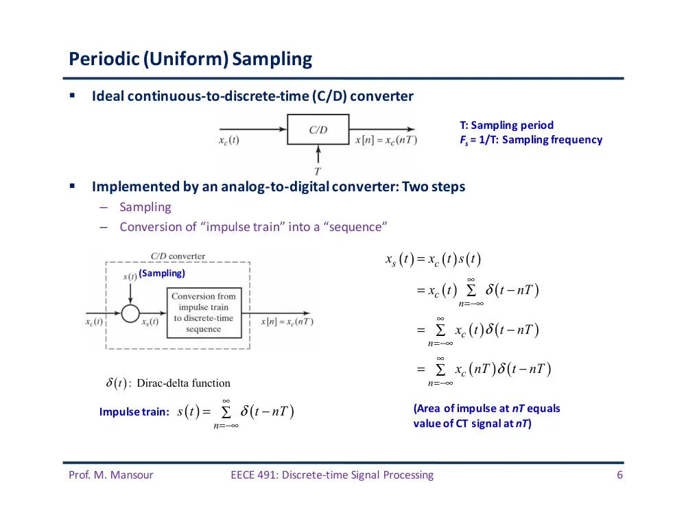Mansour EECE 491: Discrete-­‐time Signal Processing 6 Periodic (Uniform) Sampling § Ideal continuous-­‐to-­‐discrete-­‐time (C/D) converter § Implemented by an analog-­‐to-­‐digital converter: Two steps – Sampling – Conversion of “impulse train” into a “sequence” ( ) ( ) n s t t nT δ ∞ =−∞ = − ∑ T: Sampling period Fs = 1/T: Sampling frequency Impulse train: � ( ) ( ) ( ) ( ) ( ) ( ) ( ) ( ) ( ) s c c n c n c n x t x t s t x t t nT x t t nT x nT t nT δ δ δ ∞ =−∞ ∞ =−∞ ∞ =−∞ = = − ∑ = − ∑ = − ∑ (Sampling) ( ): Dirac-delta function t δ (Area of impulse at nT equals value of CT signal at nT) Prof. M. Mansour EECE 491: Discrete-­‐time Signal Processing 7 Periodic Sampling Prof. M. 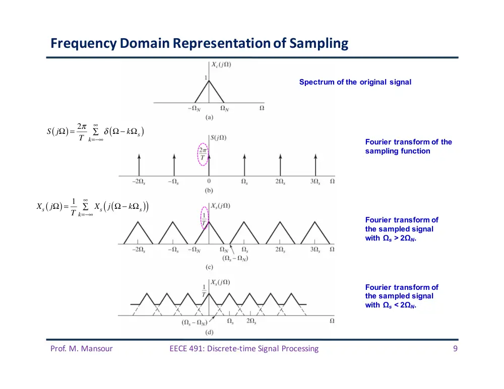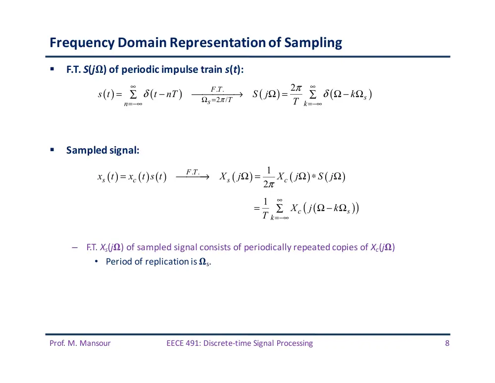Mansour EECE 491: Discrete-­‐time Signal Processing 8 Frequency Domain Representation of Sampling § F.T. S(j𝛀) of periodic impulse train s(t): § Sampled signal: – F.T. Xs(j𝛀) of sampled signal consists of periodically repeated copies of Xc(j𝛀) • Period of replication is 𝛀s. ( ) ( ) ( ) ( ) . . 2 / 2 F T s T s n k s t t nT S j k T π π δ δ ∞ ∞ Ω = =−∞ =−∞ = − ⎯⎯⎯⎯→ Ω = Ω − Ω ∑ ∑ ( ) ( ) ( ) ( ) ( ) ( ) . . 1 2 F T s c s c x t x t s t X j X j S j π = ⎯⎯⎯→ Ω = Ω ∗ Ω ( ) ( ) 1 c s k X j k T ∞ =−∞ = Ω − Ω ∑ Prof. M. Mansour EECE 491: Discrete-­‐time Signal Processing 9 Frequency Domain Representation of Sampling Spectrum  of  the  original  signal Fourier  transform  of  the sampling  function Fourier  transform  of the  sampled  signal with  Ωs >  2ΩN. Fourier  transform  of the  sampled  signal with  Ωs <  2ΩN. S jΩ ( ) = 2π T δ Ω − kΩs ( ) k=−∞ ∞ ∑ Xs jΩ ( ) = 1 T Xs j Ω − kΩs ( ) ( ) k=−∞ ∞ ∑ Prof. M. 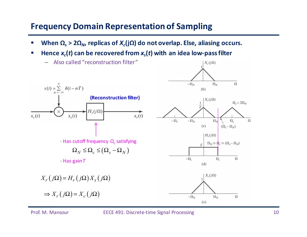Mansour EECE 491: Discrete-­‐time Signal Processing 10 Frequency Domain Representation of Sampling § When Ωs > 2ΩN, replicas of Xc(jΩ) do not overlap. Else, aliasing occurs. § Hence xc(t) can be recovered from xs(t) with an idea low-­‐pass filter – Also called “reconstruction filter” -­‐ Has cutoff frequency Ωc satisfying ( ) N c s N Ω ≤ Ω ≤ Ω − Ω -­‐ Has gain T ( ) ( ) ( ) r r s X j H j X j Ω = Ω Ω ( ) ( ) r c X j X j ⇒ Ω = Ω (Reconstruction filter) Prof. M. Mansour EECE 491: Discrete-­‐time Signal Processing 11 Example 1: Impact of Aliasing ( ) ( ) ( ) ( ) 0 0 0 cos c c x t t X j πδ πδ = Ω Ω = Ω − Ω + Ω + Ω 0 0 Two cases: 2 2 s s Ω > Ω Ω < Ω ( ) ( ) 0 cos r c x t x t t ⇒ = = Ω ( ) ( ) ( 0 ) cos r c s x t x t t ⇒ = = Ω − Ω Prof. M. Mansour EECE 491: Discrete-­‐time Signal Processing 12 Frequency Domain Representation of Sampling Prof. M. Mansour EECE 491: Discrete-­‐time Signal Processing 13 Frequency Domain Representation of Sampling § Relationship between ( ) ( ) ( ) C.T.F.T c c X j x t Ω = ( ) ( [ ] ) =D.T.F.T X e j x n ω ( ) ( ) ( ) s c n x t x nT t nT δ ∞ =−∞ = − ∑ ( ) ( ) j Tn s c n X j x nT e ∞ − Ω =−∞ Ω = ∑ [ ] ( ) c x n x nT = ( ) [ ] j j n n X e x n e ω ω ∞ − =−∞ = ∑ ( ) ( ) ( ) j j T s T X j X e X e ω ω Ω =Ω Ω = = C.T.F.T. But: Then ( ) ( ) ( ) 1 s c s k X j X j k T ∞ =−∞ Ω = Ω − Ω ∑ We also proved ( ) ( ) ( ) 1 j T c s k X e X j k T ∞ Ω =−∞ ⇒ = Ω − Ω ∑ OR ( ) 1 2 j c k k X e X j T T T ω ω π ∞ =−∞ ⎛ ⎞ ⎛ ⎞ ⇒ = − ∑ ⎜ ⎟ ⎜ ⎟ ⎝ ⎠ ⎝ ⎠ ? Prof. M. Mansour EECE 491: Discrete-­‐time Signal Processing 14 Frequency Domain Representation of Sampling § X(ej𝝎) is a frequency-­‐scaled version of Xs(j𝛀) § Frequency scaling specified by 𝝎 = 𝛀T § Equivalent to frequency normalization: – Frequency 𝛀s in Xs(j𝛀) normalized to 𝝎 = 2𝜋 in X(ej𝜔) Prof. M. Mansour EECE 491: Discrete-­‐time Signal Processing 15 Example 2 § Sample the CT signal at T = 1/6000 and show F.T. of CT & DT signals § Solution: – Highest frequency in C.T. signal 𝛀N = 4000� – Nyquist rate 𝛀S = 12000𝜋 > 2𝛀 N= 8000� – No aliasing – F.T. ( ) cos4000 cx t πt = ( ) ( ) ( ) 4000 4000 Xc j πδ π πδ π Ω = Ω − + Ω + ( ) ( ) ( ) 1 s c s k X j X j k T ∞ =−∞ ⇒ Ω = Ω − Ω ∑ Has gain T Has cutoff frequency 𝛀c satisfying / 2 c Ω = Ωs Prof. M. Mansour EECE 491: Discrete-­‐time Signal Processing 16 Example 2 (cont’d) § Repeat for – Nyquist rate not satisfied since 𝛀S = 12000𝜋 < 2 𝛀N = 32000𝜋 � – Aliasing occurs ( ) cos16000 cx t πt = Prof. M. Mansour EECE 491: Discrete-­‐time Signal Processing 17 Reconstruction of a Band-­‐limited Signal from its Samples Prof. M. Mansour EECE 491: Discrete-­‐time Signal Processing 18 Reconstruction of a Band-­‐limited Signal from its Samples § Given a sequence of samples , can we recover the original signal ? § First form an impulse train in which successive samples are assigned an area equal to § Pass this signal thru an ideal low-­‐pass C.T. filter with frequency response and impulse response [ ] x n ( ) [ ] ( ) s n x t x n t nT δ ∞ =−∞ = − ∑ cx ( ) t sx ( ) t [ ] x n ( ) Hr jΩ rh ( ) t ( ) [ ] ( ) r r n x t x n h t nT ∞ =−∞ = − ∑ -­‐ Hr(j𝛀) has cutoff frequency 𝛀c satisfying ( ) N c s N Ω ≤ Ω ≤ Ω − Ω -­‐ Hr(j𝛀) has gain T -­‐ Convenient choice of 𝛀c is 𝛀 s /2 Prof. M. Mansour EECE 491: Discrete-­‐time Signal Processing 19 Reconstruction of a Band-­‐limited Signal from its Samples § The impulse response of the ideal LPF with cutoff frequency 𝛀c = 𝛀s /2 = 𝝅/T is: § Then: § Note that: – hr(0) = 1 – hr(nT) = 0, for n = �1, �2, … – Then if x[n] = xr(nT) è xr(mT) = xc(mT) for all integer values of m. – Therefore, reconstructed signal xr(t) has same values as the original signal xc(t) at the sampling times, independently of T. § The ideal LPF “interpolates” between the impulses xs(t) to construct xc(t) ( ) [ ] ( ) ( ) sin / / r n t nT T x t x n t nT T π π ∞ =−∞ − ⎡ ⎤ ⎣ ⎦ = ∑ − ( ) ( ) sin / / r t T h t t T π π = Prof. M. Mansour EECE 491: Discrete-­‐time Signal Processing 20 Reconstruction of a Band-­‐limited Signal from its Samples [ ] ( ) ( ) sin / / t nT T x n t nT T π π − ⎡ ⎤ ⎣ ⎦ − Prof. M. Mansour EECE 491: Discrete-­‐time Signal Processing 21 Ideal Discrete-­‐to-­‐Continuous-­‐Time (D/C) Converter In frequency domain: ( ) [ ] ( ) r r n x t x n h t nT ∞ =−∞ = − ⇒ ∑ ( ) [ ] ( ) ( ) [ ] ( ) ( ) j Tn r r n j Tn r n j T r X j x n H j e H j x n e H j X e ∞ − Ω =−∞ ∞ − Ω =−∞ Ω Ω = Ω ∑ = Ω ∑ = Ω Prof. M. Mansour EECE 491: Discrete-­‐time Signal Processing 22 D.T. Processing of C.T. Signals Prof. M. Mansour EECE 491: Discrete-­‐time Signal Processing 23 D.T. Processing of C.T. Signals ( ) 1 2 j c k k X e X j T T T ω ω π ∞ =−∞ ⎛ ⎞ ⎛ ⎞ = − ∑ ⎜ ⎟ ⎜ ⎟ ⎝ ⎠ ⎝ ⎠ [ ] ( ) c x n x nT = ( ) Xc jΩ ( ) j X e ω ( ) j Y e ω ( ) rY jΩ [ ] h n ( ) j H e ω ( ) [ ] ( ) ( ) sin / / r n t nT T y t y n t nT T π π ∞ =−∞ − ⎡ ⎤ ⎣ ⎦ = ∑ − ( ) ( ) ( ) ( ) / 0 j j r r TY e T Y j H j Y e otherwise π Ω Ω ⎧ Ω < ⎪ Ω = Ω = ⎨ ⎪⎩ ( ) ( ) ( ) j j j Y e H e X e ω ω ω = [ ] [ ] [ ] y n x n h n = ∗ If DT system is LTI ( ) ( ) ( ) r eff c Y j H j X j Ω = Ω Ω Prof. M. Mansour EECE 491: Discrete-­‐time Signal Processing 24 D.T. Processing of C.T. Signals: D.T. System is LTI § Overall C.T. system is equivalent to an LTI system whose effective frequency response is – Conditions: • Input signal is band-­‐limited + sampling rate > Nyquist rate (to avoid aliasing) • C/D is ideal • D.T. system is LTI • D/C is ideal § Proof: ( ) ( ) ( ) D.T. system is LTI j j j Y e H e X e ω ω ω ⇒ = ( ) ( ) ( ) r eff c Y j H j X j Ω = Ω Ω ( ) ( ) ( ) ( ) ( ) ( ) D/C is ideal j T j T j T r r r Y j H j Y e H j H e X e Ω Ω Ω ⇒ Ω = Ω = Ω Relating X(ejΩT) to Xc(jΩ) thru sampling � ( ) ( ) ( ) 1 2 j T r r c k k Y j H j H e X j T T π ∞ Ω =−∞ ⎛ ⎞ ⎛ ⎞ Ω = Ω Ω − ∑ ⎜ ⎟ ⎜ ⎟ ⎝ ⎠ ⎝ ⎠ ( ) input bandlimited 0 for / Xc j π T ⇒ Ω = Ω > ( ) ideal with cutoff / , gain 1/ r c H j T T π Ω Ω = + ( ) ( ) ( ) / 0 / j j c r H e X e T Y j T π π Ω Ω ⎧ Ω < ⎪ Ω = ⎨ Ω ≥ ⎪⎩ ( ) ( ) ( ) r eff c Y j H j X j Ω = Ω Ω ( ) ( ) / 0 / j eff H e T H j T π π Ω ⎧ Ω < ⎪ Ω = ⎨ Ω ≥ ⎪⎩ � Prof. M. Mansour EECE 491: Discrete-­‐time Signal Processing 25 Example 3 § Consider a discrete-­‐time LTI system with § For band-­‐limited inputs sampled above the Nyquist rate, the overall C.T. system will behave as an LTI C.T. system with frequency response ( ) 1 0 c j c H e ω ω ω ω ω < ⎧ = ⎨ ≥ ⎩ ( ) 1 or /T 0 or /T c c eff c c T H j T ω ω ω ω Ω < Ω < ⎧ Ω = ⎨ Ω ≥ Ω ≥ ⎩ periodic Has cutoff frequency ωc/T D.T. Filter C.T. Filter Prof. M. Mansour EECE 491: Discrete-­‐time Signal Processing 26 Example 3 (cont’d) (a)  F.T.  of  a  band-­limited  input  signal. (b)  F.T.  of  sampled  input  plotted  as  a function  of  C.T.  frequency  Ω. (c)  F.T.  X  (ejω)  of  sequence  of  samples  and frequency  response  H(ejω)  of  D.T.  system plotted  versus  ω. (d)  F.T.  of  output  of  D.T.  system. (e)  F.T.  of  output  of  D.T.  system  and frequency  response  of  ideal  reconstruction filter  plotted  versus  Ω. (f)  F.T.  of  output. No  aliasing: ( ) 2 N c T π ω − Ω ≥ Prof. M. Mansour EECE 491: Discrete-­‐time Signal Processing 27 Example 3 (cont’d) § The effective filter below still holds even if aliasing occurs, provided aliased or distorted components are eliminated by D.T. filter H(ej𝝎) ( ) 1 or /T 0 or /T c c eff c c T H j T ω ω ω ω Ω < Ω < ⎧ Ω = ⎨ Ω ≥ Ω ≥ ⎩ No  aliasing: ( ) 2 N c T π ω − Ω ≥ Nyquist  condition: ( ) 2 N N T T π − Ω ≥ Ω Prof. M. Mansour EECE 491: Discrete-­‐time Signal Processing 28 Example 4: D.T. Implementation of an Ideal C.T. Differentiator § Ideal C.T. differentiator is defined by § We want to realize this filter using a C/D converter, D.T. filter, D/C converter – Inputs are band-­‐limited – Equivalent effective C.T. filter becomes § D.T. filter then become § Impulse response: ( ) ( ) c c d y t x t = dt ⎡ ⎤ ⎣ ⎦ ( ) Hc j j Ω = Ω ( ) ( ), / , /T 0, /T 0, / j eff H e T j H j T π π π π Ω ⎧ Ω < Ω Ω < ⎧ ⎪ Ω = = ⎨ ⎨ Ω ≥ Ω ≥ ⎩ ⎪⎩ ( ) , j j H e T ω ω ω π = < [ ] 2 1 2 cos sin 0 0 cos 0 j n j h n e d T n n n n T n n n nT π ω π ω ω π π π π π π − ⎛ ⎞ = ∫ ⎜ ⎟ ⎝ ⎠ − = = ⎧⎪ = ⎨ ≠ ⎪⎩ Apply 'Hôpital's rule Prof. M. Mansour EECE 491: Discrete-­‐time Signal Processing 29 Example 4: D.T. Implementation of an Ideal C.T. Differentiator ( ) , /T 0, /T eff j H j π π Ω Ω < ⎧ Ω = ⎨ Ω ≥ ⎩ ( ) , j j H e T ω ω ω π = < Prof. M. Mansour EECE 491: Discrete-­‐time Signal Processing 30 Impulse Invariance (Revisited) § Given a desired C.T. we wish to implement using a D.T. system as follows: Prof. M. Mansour EECE 491: Discrete-­‐time Signal Processing 31 Impulse Invariance (Revisited) § With Hc(j�) band-­‐limited, we choose H(ej�) so that: § What is resulting relationship between hc(t) and h[n]? – h[n] is a scaled, sampled version of hc(t), under the impulse invariance condition ( ) ( ) ( ) ( ) / , eff c j c H j H j H e H j T ω ω ω π Ω = Ω ⇒ = < Also ( ) 0, / Hc j π T Ω = Ω ≥ [ ] ( ) if c h n h nT = ( ) 1 2 then j c k k H e H j T T T ω ω π ∞ =−∞ ⎛ ⎞ ⎛ ⎞ = − ∑ ⎜ ⎟ ⎜ ⎟ ⎝ ⎠ ⎝ ⎠ ( ) But: 0, / Hc j π T Ω = Ω ≥ ( ) 1 Therefore, , j c H e H j T T ω ω ω π ⎛ ⎞ = < ⎜ ⎟ ⎝ ⎠ ( ) [ ] [ ] ( ) So to get for , we scale so that j c c H e H j h n h n T h nT T ω ω ω π ⎛ ⎞ = < = ⋅ ⎜ ⎟ ⎝ ⎠ Prof. M. Mansour EECE 491: Discrete-­‐time Signal Processing 32 Example 5: D.T. LPF Obtained by Impulse Invariance § Design an ideal D.T. LPF with cutoff frequency 𝛚c < 𝝅 by sampling a C.T. LPF with cutoff frequency 𝛀c. § Solution: We have § The cutoff frequency 𝛚c is related to 𝛀c by § Impulse response of C.T. LPF is § Using impulse invariance, we obtain ( ) 1, 0, c c c H j Ω < Ω ⎧ Ω = ⎨ Ω ≥ Ω ⎩ c cT ω = Ω ( ) sin c c t h t πt Ω = [ ] ( ) ( ) ( ) sin sin c c c h n T h nT nT T nT n n π ω π = ⋅ Ω = = ( ) 1, 0, c j c H e ω ω ω ω ω π < ⎧ ⇒ = ⎨ ≤ ≤ ⎩ Prof. M. Mansour EECE 491: Discrete-­‐time Signal Processing 33 C.T. Processing of D.T. Signals Prof. M. Mansour EECE 491: Discrete-­‐time Signal Processing 34 C.T. Processing of D.T. Signals § From definitions of D/C and C/D, we must have Xc(j𝛀)=0, Yc(j𝛀)=0 for |𝛀| ≥ 𝝅/T § In frequency domain: ( ) [ ] ( ) ( ) sin / / c n t nT T x t x n t nT T π π ∞ =−∞ − ⎡ ⎤ ⎣ ⎦ = ∑ − ( ) ( ) ( ) ( ) ( ) ( ) , / 1 , j T c c c c j c X j TX e T Y j H j X j Y e Y j T T ω π ω ω π Ω Ω = Ω < Ω = Ω Ω ⎛ ⎞ = < ⎜ ⎟ ⎝ ⎠ ( ) , j c H e H j T ω ω ω π ⎛ ⎞ ⇒ = < ⎜ ⎟ ⎝ ⎠ ( ) ( ) or , / j T Hc j H e T π Ω Ω = Ω < Prof. M. Mansour EECE 491: Discrete-­‐time Signal Processing 35 Example 6: Non-­‐Integer Delay § Consider a D.T. system with frequency response: § We seek an interpretation in the C.T. domain. § Choose a C.T. filter with response: – Here, xc(t) is band-­‐limited interpolation of x[n]; y[n] is obtained by sampling yc(t) § Example: if 𝚫=1/2, y[n] would be the band-­‐limited interpolation halfway between the input sequence values. ( ) [ ] [ ] , , not necessarily an integer j j H e e y n x n ω ω ω π − Δ = < = − Δ Δ ( ) ( ) ( ) ( ) j T j T c c c H j H e e y t x t T Ω − Ω Δ Ω = = = − Δ [ ] ( ) ( ) [ ] ( ) ( ) [ ] ( ) ( ) sin / / sin c c k t nT k y n y nT x nT T t T kT T x k t T kT T n k x k n k π π π π ∞ =−∞ = ∞ =−∞ = = − Δ − Δ − ⎡ ⎤ ⎣ ⎦ = ∑ − Δ − − − Δ ⎡ ⎤ ⎣ ⎦ = ∑ − − Δ [ ] ( ) ( ) sin n x n n π π − Δ ⎡ ⎤ ⎣ ⎦ ≡ ∗ − Δ Prof. M. Mansour EECE 491: Discrete-­‐time Signal Processing 36 Example 6: Non-­‐Integer Delay (a)  C.T.  processing  of  the  D.T.  sequence  (b)  can  produce  a  new  sequence  with  a  “half-­ sample”  delay. Prof. M. Mansour EECE 491: Discrete-­‐time Signal Processing 37 Example 7: Moving-­‐Average System with Non-­‐Integer Delay § For an (M+1)-­‐point causal moving average system, we have § Can represent as a cascade of two systems: § If M is even, then linear phase term is an integer delay § If M is odd, then linear phase term is a non-­‐integer delay (integer-­‐plus-­‐one-­‐half) – y[n] is then the band-­‐limited interpolation of w[n] – Followed by a C.T. delay of MT/2, where T is sampling period of D/C interpolation of w[n]) – Followed by C/D conversion with sampling period T. ( ) ( ) ( ) /2 sin 1 / 2 1 , 1 sin / 2 j j M M H e e M ω ω ω ω π ω − + ⎡ ⎤ ⎣ ⎦ = < + Prof. M. Mansour EECE 491: Discrete-­‐time Signal Processing 38 Example 7 (cont’d) Illustration of moving-­‐average filtering. (a) Input signal x[n] = cos(0.25πn). (b) Corresponding output of six-­‐point moving-­‐average filter. M = 5 Prof. M. Mansour EECE 491: Discrete-­‐time Signal Processing 39 Example 7 (cont’d) [ ] ( ) 0.25 0.25 1 1 cos 0.25 2 2 j n j n x n n e e π π π − = = + ( ) ( ) ( ) /2 sin 1 / 2 1 , 1 sin / 2 j j M M H e e M ω ω ω ω π ω − + ⎡ ⎤ ⎣ ⎦ = < + [ ] ( ) ( ) ( ) 0.25 0.25 0.25 0.25 1 1 2 2 0.308cos 0.25 2.5 j j n j j n y n H e e H e e n π π π π π − − = + = − ⎡ ⎤ ⎣ ⎦ Moving average filter: • Reduces amplitude of input • Introduces a phase shift corresponding to 2.5 samples of delay