MATH 218 Chapter Summary, Fall 2011

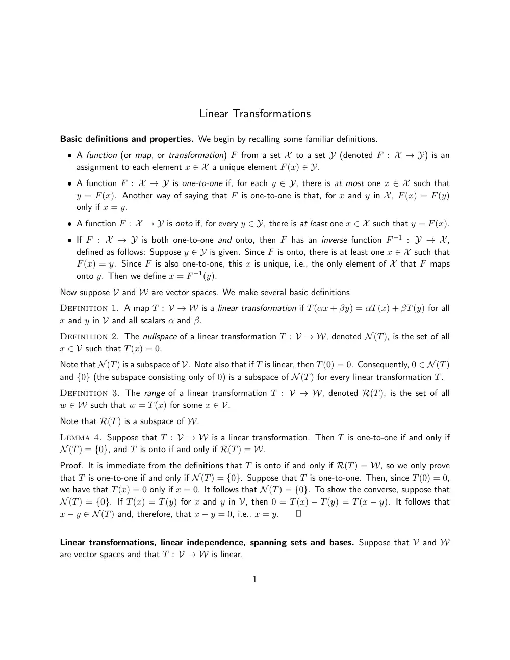
Linear Transformations Basic definitions and properties. We begin by recalling some familiar definitions. • A function (or map, or transformation) F from a set X to a set Y (denoted F : X → Y) is an assignment to each element x ∈ X a unique element F(x) ∈ Y. • A function F : X → Y is one-to-one if, for each y ∈ Y, there is at most one x ∈ X such that y = F(x). Another way of saying that F is one-to-one is that, for x and y in X, F(x) = F(y) only if x = y. • A function F : X → Y is onto if, for every y ∈ Y, there is at least one x ∈ X such that y = F(x). • If F : X → Y is both one-to-one and onto, then F has an inverse function F −1 : Y → X, defined as follows: Suppose y ∈ Y is given. Since F is onto, there is at least one x ∈ X such that F(x) = y. Since F is also one-to-one, this x is unique, i.e., the only element of X that F maps onto y. Then we define x = F −1(y). Now suppose V and W are vector spaces. We make several basic definitions Definition 1. A map T : V → W is a linear transformation if T(αx + βy) = αT(x) + βT(y) for all x and y in V and all scalars α and β. Definition 2. The nullspace of a linear transformation T : V → W, denoted N(T), is the set of all x ∈ V such that T(x) = 0. Note that N(T) is a subspace of V. Note also that if T is linear, then T(0) = 0. Consequently, 0 ∈ N(T) and {0} (the subspace consisting only of 0) is a subspace of N(T) for every linear transformation T. Definition 3. The range of a linear transformation T : V → W, denoted R(T), is the set of all w ∈ W such that w = T(x) for some x ∈ V. Note that R(T) is a subspace of W. Lemma 4. Suppose that T : V → W is a linear transformation. Then T is one-to-one if and only if N(T) = {0}, and T is onto if and only if R(T) = W. Proof. It is immediate from the definitions that T is onto if and only if R(T) = W, so we only prove that T is one-to-one if and only if N(T) = {0}. Suppose that T is one-to-one. Then, since T(0) = 0, we have that T(x) = 0 only if x = 0. It follows that N(T) = {0}. To show the converse, suppose that N(T) = {0}. If T(x) = T(y) for x and y in V, then 0 = T(x) − T(y) = T(x − y). It follows that x − y ∈ N(T) and, therefore, that x − y = 0, i.e., x = y. Linear transformations, linear independence, spanning sets and bases. Suppose that V and W are vector spaces and that T : V → W is linear. 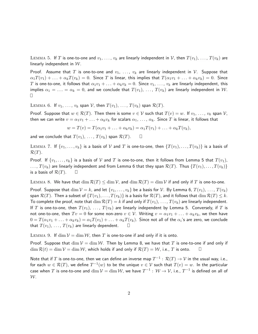1 Lemma 5. If T is one-to-one and v1, . . . , vk are linearly independent in V, then T(v1), . . . , T(vk) are linearly independent in W. Proof. Assume that T is one-to-one and v1, . . . , vk are linearly independent in V. Suppose that α1T(v1) + . . . + αkT(vk) = 0. Since T is linear, this implies that T(α1v1 + . . . + αkvk) = 0. Since T is one-to-one, it follows that α1v1 + . . . + αkvk = 0. Since v1, . . . , vk are linearly independent, this implies α1 = . . . = αk = 0, and we conclude that T(v1), . . . , T(vk) are linearly independent in W. Lemma 6. If v1, . . . , vk span V, then T(v1), . . . , T(vk) span R(T). Proof. Suppose that w ∈ R(T). Then there is some v ∈ V such that T(v) = w. If v1, . . . , vk span V, then we can write v = α1v1 + . . . + αkvk for scalars α1, . . . , αk. Since T is linear, it follows that w = T(v) = T(α1v1 + . . . + αkvk) = α1T(v1) + . . . + αkT(vk), and we conclude that T(v1), . . . , T(vk) span R(T). Lemma 7. If {v1, . . . , vk} is a basis of V and T is one-to-one, then {T(v1), . . . , T(vk)} is a basis of R(T). Proof. If {v1, . . . , vk} is a basis of V and T is one-to-one, then it follows from Lemma 5 that T(v1), . . . , T(vk) are linearly independent and from Lemma 6 that they span R(T). Thus {T(v1), . . . , T(vk)} is a basis of R(T). Lemma 8. We have that dim R(T) ≤ dim V, and dim R(T) = dim V if and only if T is one-to-one. Proof. Suppose that dim V = k, and let {v1, . . . , vk} be a basis for V. By Lemma 6, T(v1), . . . , T(vk) span R(T). Then a subset of {T(v1), . . . , T(vk)} is a basis for R(T), and it follows that dim R(T) ≤ k. To complete the proof, note that dim R(T) = k if and only if T(v1), . . . , T(vk) are linearly independent. If T is one-to-one, then T(v1), . . . , T(vk) are linearly independent by Lemma 5. Conversely, if T is not one-to-one, then Tv = 0 for some non-zero v ∈ V. Writing v = α1v1 + . . . + αkvk, we then have 0 = T(α1v1 + . . . + αkvk) = α1T(v1) + . . . + αkT(vk). Since not all of the αi’s are zero, we conclude that T(v1), . . . , T(vk) are linearly dependent. Lemma 9. If dim V = dim W, then T is one-to-one if and only if it is onto. Proof. Suppose that dim V = dim W. Then by Lemma 8, we have that T is one-to-one if and only if dim R(t) = dim V = dim W, which holds if and only if R(T) = W, i.e., T is onto. Note that if T is one-to-one, then we can define an inverse map T −1 : R(T) → V in the usual way, i.e., for each w ∈ R(T), we define T −1(w) to be the unique v ∈ V such that T(v) = w. In the particular case when T is one-to-one and dim V = dim W, we have T −1 : W → V, i.e., T −1 is defined on all of W. 2 Examples. 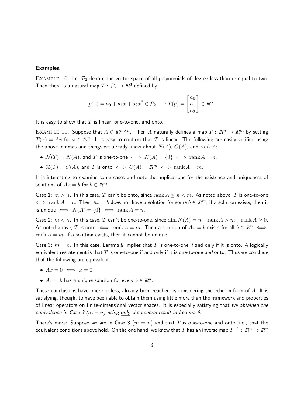Example 10. Let P2 denote the vector space of all polynomials of degree less than or equal to two. Then there is a natural map T : P2 → IR3 defined by p(x) = a0 + a1x + a2x2 ∈ P2 −→ T(p) =   a0 a1 a2   ∈ IR3. It is easy to show that T is linear, one-to-one, and onto. Example 11. Suppose that A ∈ IRm×n. Then A naturally defines a map T : IRn → IRm by setting T(x) = Ax for x ∈ IRn. It is easy to confirm that T is linear. The following are easily verified using the above lemmas and things we already know about N(A), C(A), and rank A: • N(T) = N(A), and T is one-to-one ⇐⇒ N(A) = {0} ⇐⇒ rank A = n. • R(T) = C(A), and T is onto ⇐⇒ C(A) = IRm ⇐⇒ rank A = m. It is interesting to examine some cases and note the implications for the existence and uniqueness of solutions of Ax = b for b ∈ IRm. Case 1: m > n. In this case, T can’t be onto, since rank A ≤ n < m. As noted above, T is one-to-one ⇐⇒ rank A = n. Then Ax = b does not have a solution for some b ∈ IRm; if a solution exists, then it is unique ⇐⇒ N(A) = {0} ⇐⇒ rank A = n. Case 2: m < n. In this case, T can’t be one-to-one, since dim N(A) = n − rank A > m − rank A ≥ 0. As noted above, T is onto ⇐⇒ rank A = m. Then a solution of Ax = b exists for all b ∈ IRn ⇐⇒ rank A = m; if a solution exists, then it cannot be unique. Case 3: m = n. In this case, Lemma 9 implies that T is one-to-one if and only if it is onto. A logically equivalent restatement is that T is one-to-one if and only if it is one-to-one and onto. Thus we conclude that the following are equivalent: • Ax = 0 ⇐⇒ x = 0. • Ax = b has a unique solution for every b ∈ IRn. These conclusions have, more or less, already been reached by considering the echelon form of A. It is satisfying, though, to have been able to obtain them using little more than the framework and properties of linear operators on finite-dimensional vector spaces. It is especially satisfying that we obtained the equivalence in Case 3 (m = n) using only the general result in Lemma 9. There’s more: Suppose we are in Case 3 (m = n) and that T is one-to-one and onto, i.e., that the equivalent conditions above hold. On the one hand, we know that T has an inverse map T −1 : IRn → IRn 3 defined as follows: For each y ∈ IRn, we set T −1(y) = x, where x is the unique vector in IRn such that T(x) = y. On the other hand, since the two equivalent conditions hold, we know that A is nonsingular and therefore has an inverse matrix A−1 for which A−1A = AA−1 = I (the identity matrix). Then T −1(y) = x ⇐⇒ y = T(x) ⇐⇒ y = Ax ⇐⇒ A−1y = A−1Ax = Ix = x, and so T −1(y) = A−1y for each y ∈ IRn. 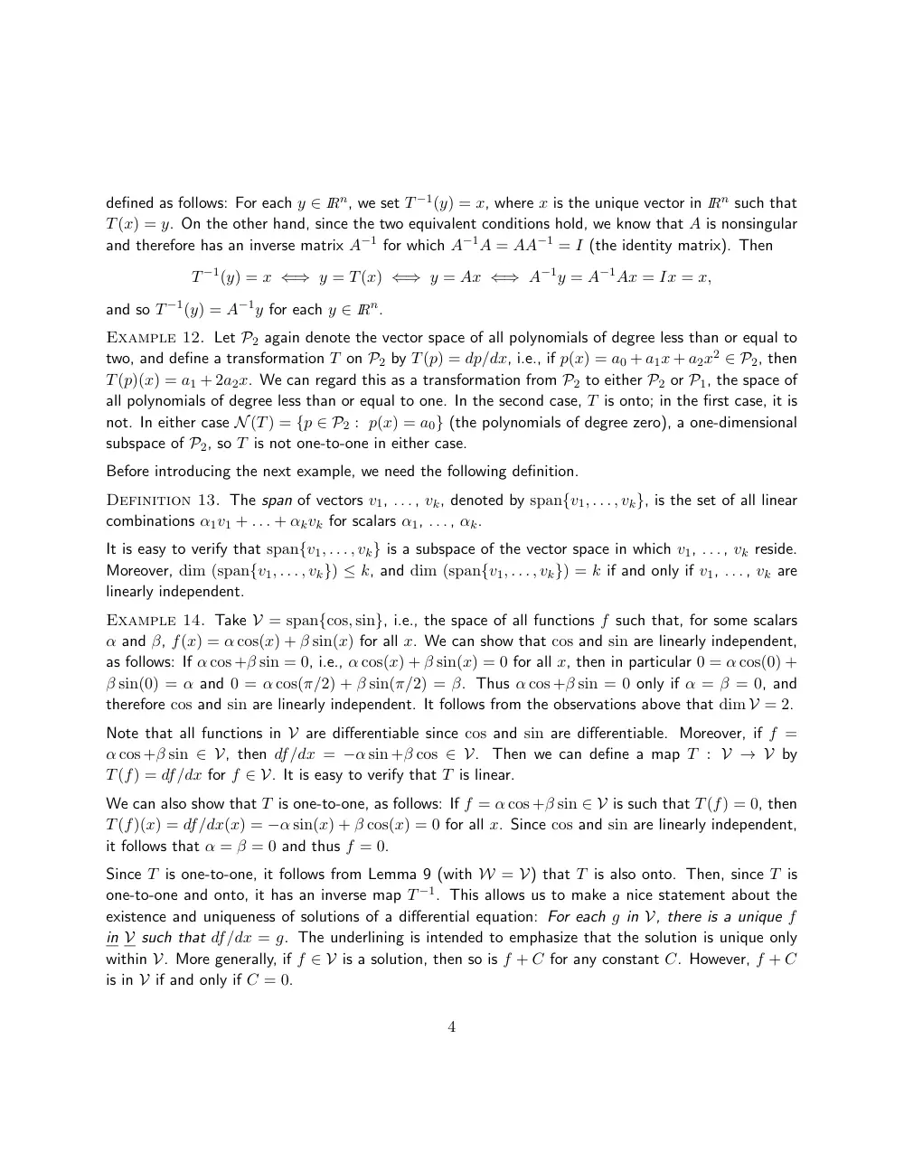Example 12. Let P2 again denote the vector space of all polynomials of degree less than or equal to two, and define a transformation T on P2 by T(p) = dp/dx, i.e., if p(x) = a0 + a1x + a2x2 ∈ P2, then T(p)(x) = a1 + 2a2x. We can regard this as a transformation from P2 to either P2 or P1, the space of all polynomials of degree less than or equal to one. In the second case, T is onto; in the first case, it is not. In either case N(T) = {p ∈ P2 : p(x) = a0} (the polynomials of degree zero), a one-dimensional subspace of P2, so T is not one-to-one in either case. Before introducing the next example, we need the following definition. Definition 13. The span of vectors v1, . . . , vk, denoted by span{v1, . . . , vk}, is the set of all linear combinations α1v1 + . . . + αkvk for scalars α1, . . . , αk. It is easy to verify that span{v1, . . . , vk} is a subspace of the vector space in which v1, . . . , vk reside. Moreover, dim (span{v1, . . . , vk}) ≤ k, and dim (span{v1, . . . , vk}) = k if and only if v1, . . . , vk are linearly independent. Example 14. Take V = span{cos, sin}, i.e., the space of all functions f such that, for some scalars α and β, f(x) = α cos(x) + β sin(x) for all x. We can show that cos and sin are linearly independent, as follows: If α cos +β sin = 0, i.e., α cos(x) + β sin(x) = 0 for all x, then in particular 0 = α cos(0) + β sin(0) = α and 0 = α cos(π/2) + β sin(π/2) = β. Thus α cos +β sin = 0 only if α = β = 0, and therefore cos and sin are linearly independent. It follows from the observations above that dim V = 2. Note that all functions in V are differentiable since cos and sin are differentiable. Moreover, if f = α cos +β sin ∈ V, then df/dx = −α sin +β cos ∈ V. Then we can define a map T : V → V by T(f) = df/dx for f ∈ V. It is easy to verify that T is linear. We can also show that T is one-to-one, as follows: If f = α cos +β sin ∈ V is such that T(f) = 0, then T(f)(x) = df/dx(x) = −α sin(x) + β cos(x) = 0 for all x. Since cos and sin are linearly independent, it follows that α = β = 0 and thus f = 0. Since T is one-to-one, it follows from Lemma 9 (with W = V) that T is also onto. Then, since T is one-to-one and onto, it has an inverse map T −1. This allows us to make a nice statement about the existence and uniqueness of solutions of a differential equation: For each g in V, there is a unique f in V such that df/dx = g. The underlining is intended to emphasize that the solution is unique only within V. More generally, if f ∈ V is a solution, then so is f + C for any constant C. However, f + C is in V if and only if C = 0. 4