MATH 218 Problems Solution Manual Chapter 1.2, Fall 2011

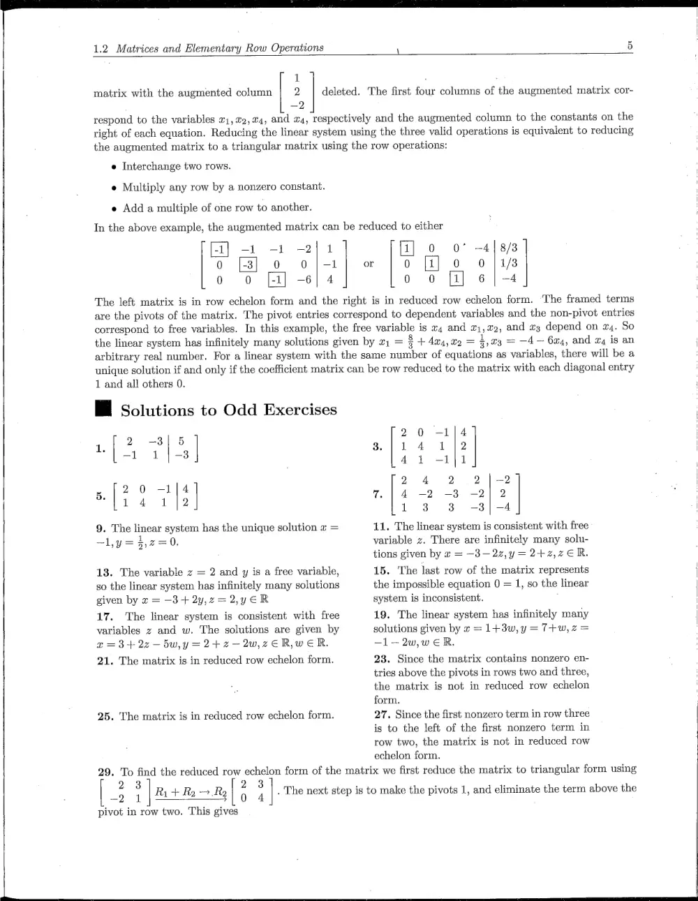
1.2 Matrices and Elementary Row Operations t 5 1 . matrix with the augmented column 2 deleted. The first four columns of the augmented matrix cor- -2 respond to the variables a1, #2,24, and x4, respectively and the augmented column to the constants on the right of each equation. Reducing the linear system using the three valid operations is equivalent to reducing the augmented matrix to a triangular matrix using the row operations: e Interchange two rows. e Multiply any row by a nonzero constant. e Add a multiple of one row to another. In the above example, the augmented matrix can be reduced to either -l} -1 -1 -2] 1 i] 0 0° -4|8/3 0 [-3] 0 oO |-1] o 0 [1] 0 0 |4/3 0 o [1] -6| 4 o o f4] 6 | -4 The left matrix is in row echelon form and the right is in reduced row echelon form. ‘The framed terms are the pivots of the matrix. The pivot entries correspond to dependent variables and the non-pivot entries correspond to free variables. In this example, the free variable is x4 and #1, 22, and «3 depend on 24. So the linear system has infinitely many solutions given by 21 = 8 + 404, %2 = 4,03 = —4— 6x4, and 24 is an arbitrary real number. For a linear system with the same number of equations as variables, there will be a unique solution if and only if the coefficient matrix can be row reduced to the matrix with each diagonal entry 1 and all others 0. WM Solutions to Odd Exercises 20 -1/4 uf 3 725 | 3/14 1/2 41 -1]1 24 2 2 |-2 rar 7 | 4 -2 -3 -2) 2 13 3 -3|-4 11. The linear system is consistent with free variable z. There are infinitely many solu- tions given by « = -3-2z,y=2+2,zER. 9. The linear system has the unique solution « = -ly=$,2=0. 13. The variable z = 2 and y is a free variable, so the linear system has infinitely many solutions given by = -34+2y,2=2,yeER 17. The linear system is consistent with free variables z and w. The solutions are given by 2 =3+2z2-5u,y=2+2-2u,zERweR. 21. The matrix is in reduced row echelon form. 25. The matrix is in reduced row echelon form. 29. To find the reduced row echelon form of the matrix we first reduce the matrix to triangular form using 2 3 2 3) | Rut Ra.Ra| § 4 2 1 pivot in row two. This gives 15. The last row of the matrix represents the impossible equation 0 = 1, so the linear system is inconsistent. 19. The linear system has infinitely many solutions given by « = 1+8w,y =7+w,z= -1—2u,weR. 23. Since the matrix contains nonzero en- tries above the pivots in rows two and three, the matrix is not in reduced row echelon form. 27. Since the first nonzero term in row three is to the left of the first nonzero term in row two, the matrix is not in reduced row echelon form. . 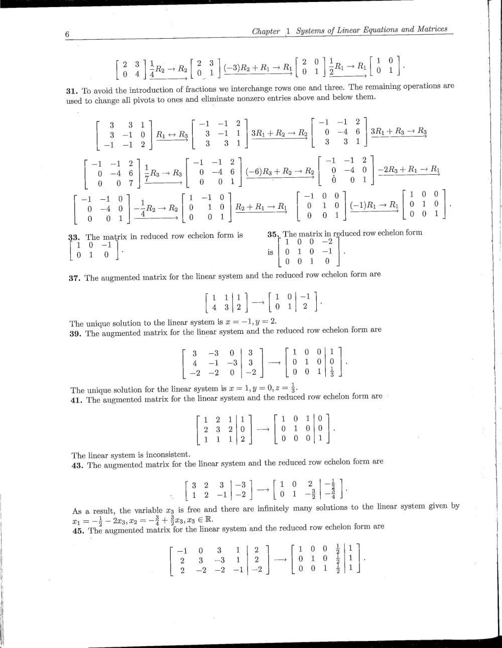The next step is to make the pivots 1, and eliminate the term above the eee 6 Chapter 1 Systems of Linear Equations and Matrices 2 38)]4 2 3 2 0)1 1 0 [3 Abie | cam rem] 5 1] Fe 4 ‘|: ne TT ————> 31. ‘To avoid the introduction of fractions we interchange rows one and three. ‘The remaining operations are used to change all pivots to ones and eliminate nonzero entries above and below them. 3 3 i -1 -1 2 -1 -1l 2 3 -1 0 | Rie Rg 3 -1 1 | 3Ri +R, Re 0 -4 6 3Ri + Rs > Rg -1 -1 2 “1 3 8 1 —"} 3 8 1] ; -1 -1 2 1 —-1 -1 2 -1 -1 2 0 -4 6 7s — Rg 0 —4 6 | (-6)R3+ Re Re 0 -4 0 —2R3+ Ri > Ry 0 oO 7 }|———~ 0 ot ; 0 ol -1 -1 0] 4 1 -1 0 -1 0 0 10 0 0 -4 0 qa > Re 0 1 0) Ro+khi > Ry 0 1 0);(-D)R- Ri); 0 1 0 0 o1};—~—+}]0 O01 0 oi; —*{£0 0 1 33. The matrix in reduced row echelon form is 35. The matrix in reduced row echelon form 10 -1 100 -2 01 0/° is| 0 1 0 -1 00 1 0 37. The augmented matrix for the linear system and the reduced row echelon form are on 1 O|-1 4 3 2 01) 2 ]° The unique solution to the linear system is a = —1,y = 2. 39. The augmented matrix for the linear system and the reduced row echelon form are 3-3 0 3 1 0 0/1 4 -1 -3)| 3 —|0 1 0/0]. -2 -2 0 |-2 0 0 143 The unique solution for the linear system is « = ly=0,2= 3 41. The augmented matrix for the linear system and the reduced row echelon form are 12 1/1 1 0 1)0 23 2/0/-—-/]0 1 0|0 1 4 142 00 Oj! The linear system is inconsistent. 43. The augmented matrix for the linear system and the reduced row echelon form are 3.2 8 |-3]_ f10 2 3 1 2 -1}-2 01 -8)-9 ]7 As a result, the variable zg is free and there are infinitely many solutions to the linear system given by Ly= -} — 293,02 = -3 + Sag, 03 ER. 45. The augmented matrix for the linear system and the reduced row echelon form are -1 0 3 1{|2 10 0 3{1 2 3 -3 1/2 |—}]0 10 3/1). 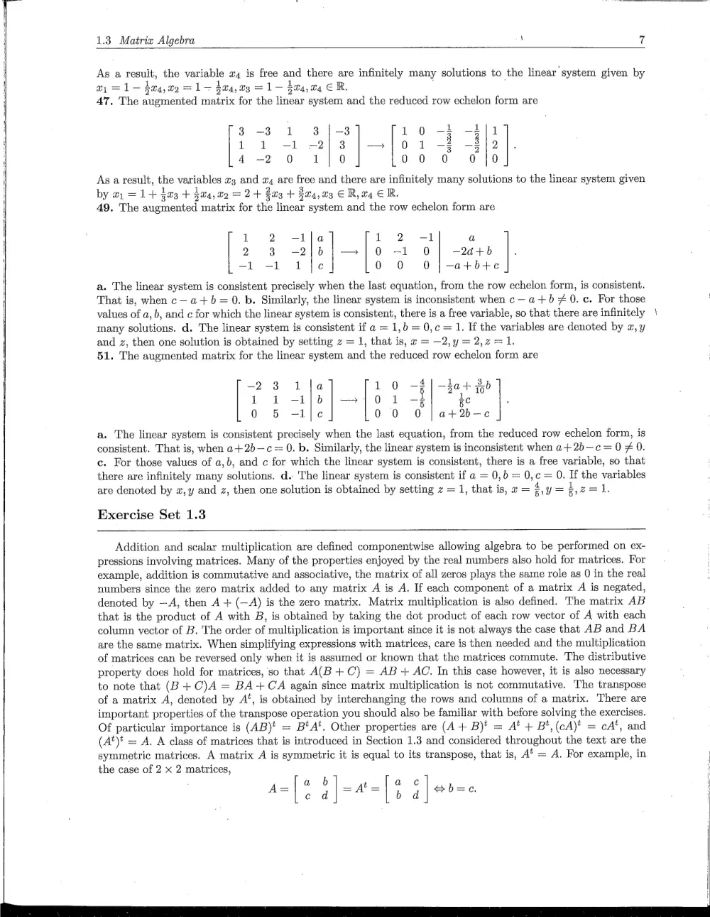2 -2 -2 -1|-2 001 4]1 1.3 Matrix Algebra \ 7 As a result, the variable x4 is free and there are infinitely many solutions to the linear’ system given by 1 1 a, =1— 404,09 = 1 $04, 03 = 1- $04,024 ER. 47. The augmented matrix for the linear system and the reduced row echelon form are 3-3 1 3 41-3 10-3 —g|1 1 1 -1 -2)3 |— {01 -% -8]2 4-2 0 1/0 00 0 0 1]0 As a result, the variables zg and a, are free and there are infinitely many solutions to the linear system given by a, = 1+ 429 + 5&4, 02 = 2+ 28 + 324,23 ER, a ER. 49. The augmented matrix for the linear system and the row echelon form are 1 2 --lja 1 2 -1 a 2 38 -2/b|—>]0 -1 O —2a+6 -1 -l Life 0 0 O |-a+b+e a. The linear system is consistent precisely when the last equation, from the row echelon form, is consistent. That is, when c—a+b=0. b. Similarly, the linear system is inconsistent when c— a+b #0. c. For those values of a,b, and c for which the linear system is consistent, there is a free variable, so that there are infinitely many solutions. d. The linear system is consistent if a = 1,b = 0,c = 1. If the variables are denoted by 2,y and z, then one solution is obtained by setting z= 1, that is, e = —2,y=2,z=1. 51. The augmented matrix for the linear system and the reduced row echelon form are -2 3 1 \a 10 -§ —ha+ 2b 1 1 -1/b | —»]0 1 -§ ze 0 5 -lle 00 0 | a+2%b-c a. The linear system is consistent precisely when the last equation, from the reduced row echelon form, is consistent. That is, when a+2b—c= 0. b. Similarly, the linear system is inconsistent when a+ 2b—c=0 4 0. c. For those values of a,b, and c for which the linear system is consistent, there is a free variable, so that there are infinitely many solutions. d. The linear system is consistent if a = 0,6 = 0,¢ = 0. If the variables are denoted by «,y and z, then one solution is obtained by setting z = 1, that is, «= $,y = $,2=1. Exercise Set 1.3 Addition and scalar multiplication are defined componentwise allowing algebra to be performed on ex- pressions involving matrices. Many of the properties enjoyed by the real numbers also hold for matrices. For example, addition is commutative and associative, the matrix of all zeros plays the same role as 0 in the real numbers since the zero matrix added to any matrix A is A. If each component of a matrix A is negated, denoted by —A, then A+ (—A) is the zero matrix. Matrix multiplication is also defined. The matrix AB that is the product of A with B, is obtained by taking the dot product of each row vector of A with each column vector of B. The order of multiplication is important since it is not always the case that AB and BA are the same matrix. When simplifying expressions with matrices, care is then needed and the multiplication of matrices can be reversed only when it is assumed or known that the matrices commute. The distributive property does hold for matrices, ‘so that A(B +C) = AB + AC. In this case however, it is also necessary to note that (B+ C)A = BA+CA again since matrix multiplication is not commutative. The transpose of a matrix A, denoted by A’, is obtained by interchanging the rows and columns of a matrix. There are important properties of the transpose operation you should also be familiar with before solving the exercises. Of particular importance is (AB)' = B'A'. Other properties are (A + B)* = A’ + B*,(cA)* = cA’, and (At)? = A. A class of matrices that is introduced in Section 1.3 and considered throughout the text are the symmetric matrices. A matrix A is symmetric it is equal to its transpose, that is, Aé = A. For example, in the case of 2 x 2 matrices, a=|¢ ifa4'= [3 g | eo=e