MECH 314 Problems 2, Spring 2014

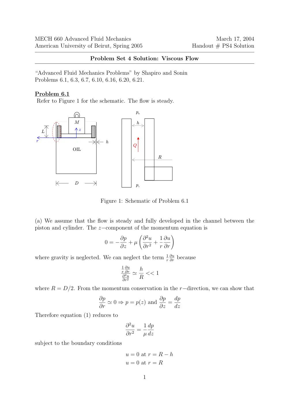
MECH 660 Advanced Fluid Mechanics March 17, 2004 American University of Beirut, Spring 2005 Handout # PS4 Solution Problem Set 4 Solution: Viscous Flow “Advanced Fluid Mechanics Problems” by Shapiro and Sonin Problems 6.1, 6.3, 6.7, 6.10, 6.16, 6.20, 6.21. Problem 6.1 Refer to Figure 1 for the schematic. The flow is steady. M OIL L h D p1 pa h Q R z r Figure 1: Schematic of Problem 6.1 (a) We assume that the flow is steady and fully developed in the channel between the piston and cylinder. The z−component of the momentum equation is 0 = −∂p ∂z + µ �∂2u ∂r2 + 1 r ∂u ∂r � where gravity is neglected. We can neglect the term 1 r ∂u ∂r because 1 r ∂u ∂r ∂2u ∂r2 ≃ h R << 1 where R = D/2. 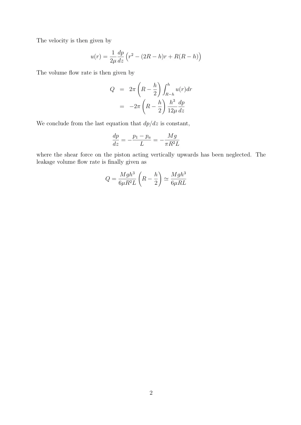From the momentum conservation in the r−direction, we can show that ∂p ∂r ≃ 0 ⇒ p = p(z) and ∂p ∂z = dp dz Therefore equation (1) reduces to ∂2u ∂r2 = 1 µ dp dz subject to the boundary conditions u = 0 at r = R − h u = 0 at r = R 1 The velocity is then given by u(r) = 1 2µ dp dz � r2 − (2R − h)r + R(R − h) � The volume flow rate is then given by Q = 2π � R − h 2 � � h R−h u(r)dr = −2π � R − h 2 � h3 12µ dp dz We conclude from the last equation that dp/dz is constant, dp dz = −p1 − pa L = − Mg πR2L where the shear force on the piston acting vertically upwards has been neglected. 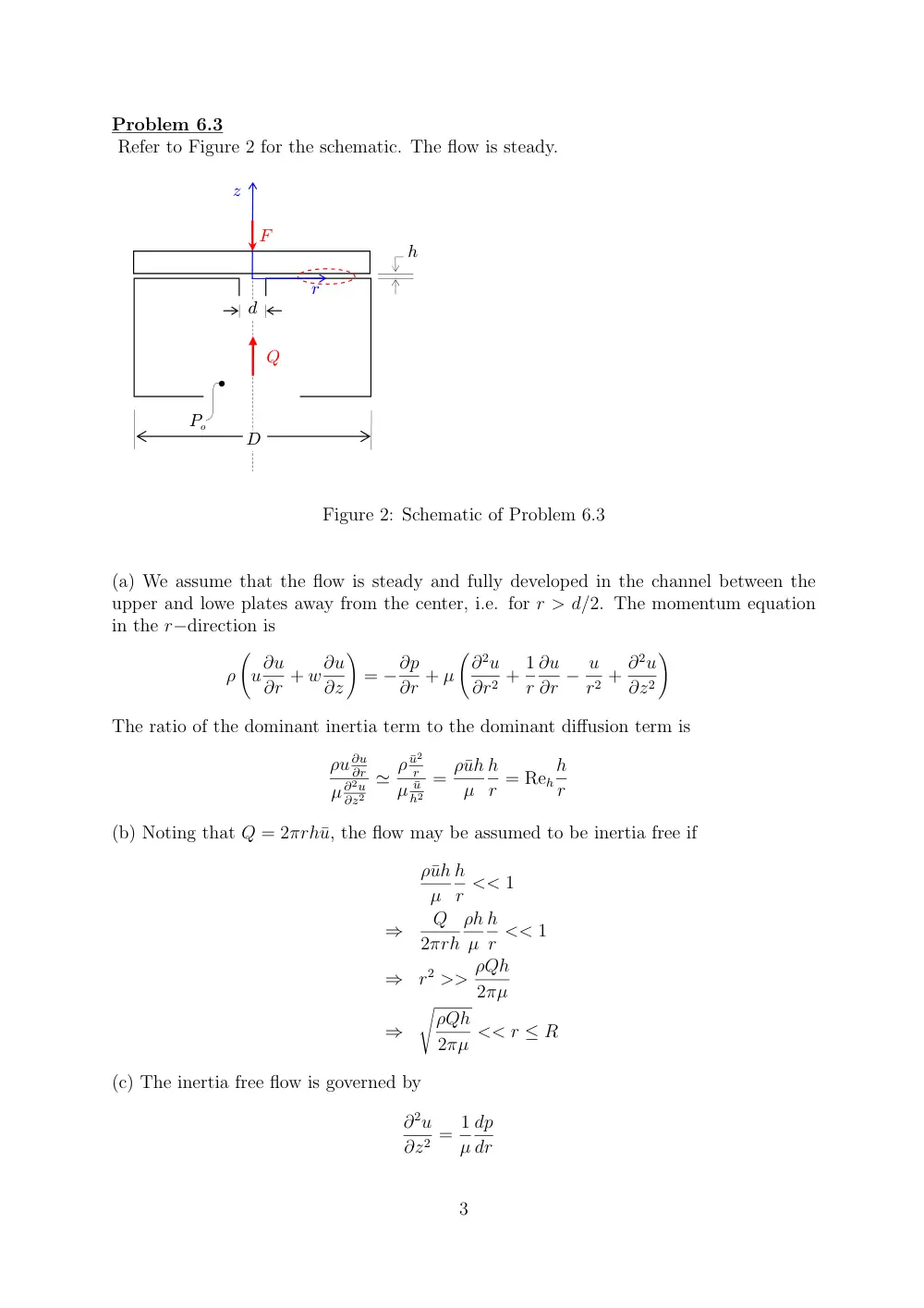The leakage volume flow rate is finally given as Q = Mgh3 6µR2L � R − h 2 � ≃ Mgh3 6µRL 2 Problem 6.3 Refer to Figure 2 for the schematic. The flow is steady. Po Q D F h d r z Figure 2: Schematic of Problem 6.3 (a) We assume that the flow is steady and fully developed in the channel between the upper and lowe plates away from the center, i.e. for r > d/2. The momentum equation in the r−direction is ρ � u∂u ∂r + w∂u ∂z � = −∂p ∂r + µ �∂2u ∂r2 + 1 r ∂u ∂r − u r2 + ∂2u ∂z2 � The ratio of the dominant inertia term to the dominant diffusion term is ρu ∂u ∂r µ ∂2u ∂z2 ≃ ρ ¯u2 r µ ¯u h2 = ρ¯uh µ h r = Reh h r (b) Noting that Q = 2πrh¯u, the flow may be assumed to be inertia free if ρ¯uh µ h r << 1 ⇒ Q 2πrh ρh µ h r << 1 ⇒ r2 >> ρQh 2πµ ⇒ � ρQh 2πµ << r ≤ R (c) The inertia free flow is governed by ∂2u ∂z2 = 1 µ dp dr 3 subject to the boundary conditions u = 0 at z = 0 u = 0 at z = h The velocity is then given by u = 1 2µ dp dr � z2 − zh � The volume flow rate is Q = 2πr 2µ dp dr � h 0 � z2 − zh � dz = −πrh3 6µ dp dr 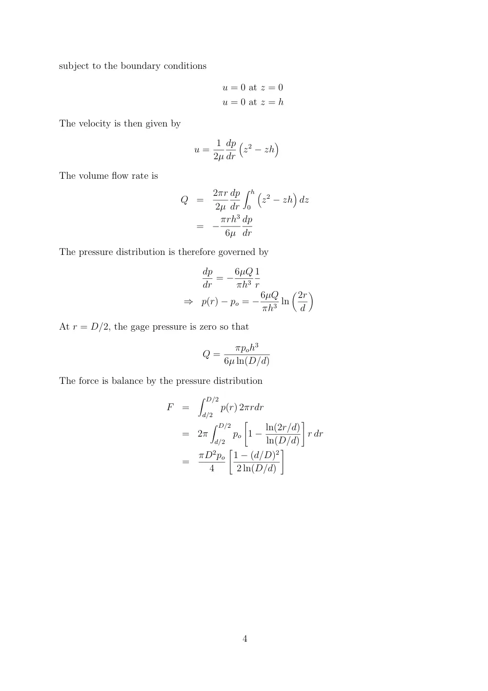The pressure distribution is therefore governed by dp dr = −6µQ πh3 1 r ⇒ p(r) − po = −6µQ πh3 ln �2r d � At r = D/2, the gage pressure is zero so that Q = πpoh3 6µ ln(D/d) The force is balance by the pressure distribution F = � D/2 d/2 p(r) 2πrdr = 2π � D/2 d/2 po � 1 − ln(2r/d) ln(D/d) � r dr = πD2po 4 �1 − (d/D)2 2 ln(D/d) � 4 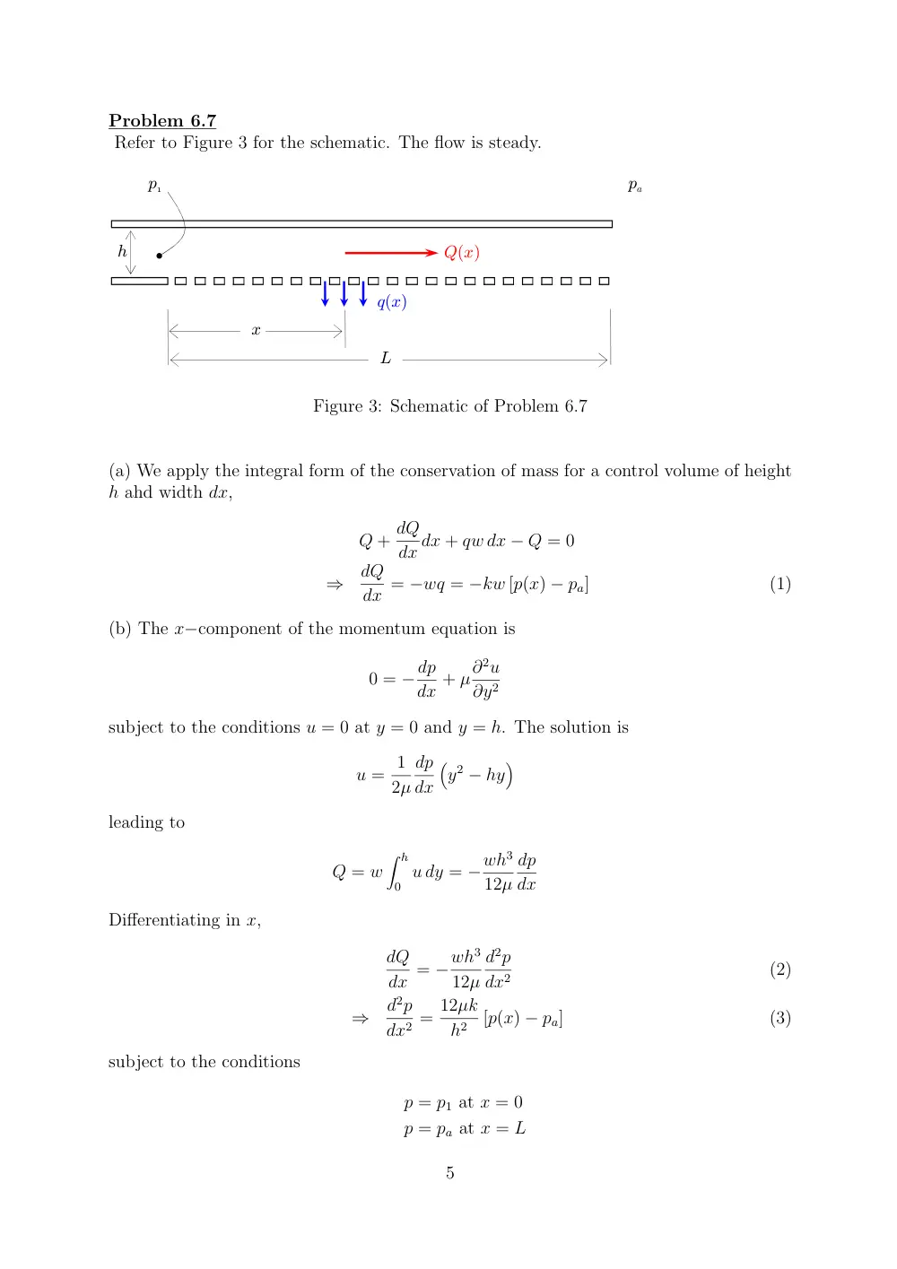Problem 6.7 Refer to Figure 3 for the schematic. The flow is steady. h pa p1 Q(x) q(x) x L Figure 3: Schematic of Problem 6.7 (a) We apply the integral form of the conservation of mass for a control volume of height h ahd width dx, Q + dQ dx dx + qw dx − Q = 0 ⇒ dQ dx = −wq = −kw [p(x) − pa] (1) (b) The x−component of the momentum equation is 0 = −dp dx + µ∂2u ∂y2 subject to the conditions u = 0 at y = 0 and y = h. The solution is u = 1 2µ dp dx � y2 − hy � leading to Q = w � h 0 u dy = −wh3 12µ dp dx Differentiating in x, dQ dx = −wh3 12µ d2p dx2 (2) ⇒ d2p dx2 = 12µk h2 [p(x) − pa] (3) subject to the conditions p = p1 at x = 0 p = pa at x = L 5 (c) In this case we have a conventional Poiseuille flow. If q is very small, then k is very small. From equation (3) d2p dx2 ≃ 0 ⇒ dp dx = pa − p1 L Therefore the location at which the gage pressure reaches half the inlet gage pressure is x∗ = L/2. (d) In this case Q(x = L) ≃ 0. A first order approximation in this xase is to assume that Q varies linearly from Q = Q0 at x = 0 to Q = 0 at x = L, dQ dx ≃ −Q0 L ⇒ Q ≃ Q0 � 1 − x L � From equation (2), wh3 12µ d2p dx2 = Q0 L Leading to the pressure distribution p(x) = 6µQ0 wh3Lx2 + �pa − p1 L − 6µQ0 wh3 � x + p1 (4) To get Q0, we integrate equation (1), 0 − Q0 = � L 0 −kw [p(x) − pa] dx ⇒ Q0 = kw � L 0 � 6µQ0 wh3Lx2 + �pa − p1 L − 6µQ0 wh3 � x + p1 − pa � dx ⇒ Q0 = wh3(p1 − pa) 2µL + 2h3/kL ≃ wh3(p1 − pa) 2µL Note kL >> h3/µL in this case. Substituting Q0 in equation (4), we get p(x) − pa p1 − pa = 3 x2 L2 − 4 x L + 1 Now we find x∗ such that (p(x∗) − pa)/(p1 − pa) = 1 2, resulting in x∗ = 0.14L. (e) The differential equation d2p∗ dx2 = αp∗(x) where p∗(x) = p(x)−pa p1−pa and α = 12µk h2 have the general solution p∗(x) = C1ex√α + C2e−x√α 6 subject to the boundary conditions p∗ = 1 at x = 0 and p∗ = 0 at x = L, we get C1 + C2 = 1 C1eL√α + C2e−L√α = 0 leading to p(x) − pa p1 − pa = e(L−x)√α − e−(L−x)√α eL√α − e−L√α • case 1: in the limit k → 0, i.e. α = 0, p(x) − pa p1 − pa = L − x L at x = L/2, we get p(x)−pa p1−pa = 1/2. • case 2: in the limit L√α >> 0, , p(x) − pa p1 − pa = e−x√α at x = ln(2) √α , we get p(x)−pa p1−pa = 1/2. 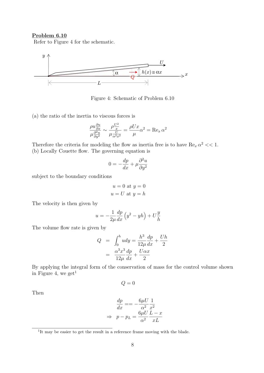7 Problem 6.10 Refer to Figure 4 for the schematic. α y x U h(x)≅ αx L Q Figure 4: Schematic of Problem 6.10 (a) the ratio of the inertia to viscous forces is ρu ∂u ∂x µ ∂2u ∂y2 ∼ ρ U2 x µ U α2x2 = ρUx µ α2 = Rex α2 Therefore the criteria for modeling the flow as inertia free is to have Rex α2 << 1. (b) Locally Couette flow. The governing equation is 0 = −dp dx + µ∂2u ∂y2 subject to the boundary conditions u = 0 at y = 0 u = U at y = h The velocity is then given by u = − 1 2µ dp dx � y2 − yh � + U y h The volume flow rate is given by Q = � h 0 udy = h3 12µ dp dx + Uh 2 = α3x3 12µ dp dx + Uαx 2 By applying the integral form of the conservation of mass for the control volume shown in Figure 4, we get1 Q = 0 Then dp dx == −6µU α2 1 x2 ⇒ p − pL = 6µU α2 L − x xL 1It may be easier to get the result in a reference frame moving with the blade. 8 Problem 6.16 Refer to Figure 5 for the schematic. viscous liquid y x h(x,t) θ g air, pa dx Figure 5: Schematic of Problem 6.16 (a) We apply conservation of mass for a control volume shown in the figure, ∂ ∂t � CV ρ dV + � CS ρu · ˆn dS = 0 ⇒ ∂ ∂t(ρh dx) + ρdQ dx dx = 0 ⇒ ∂h ∂t + dQ dx = 0 (5) where Q is the volume flowrate. The differential form of the momentum conservation in the x−direction is 0 = µ∂u2 ∂y2 + ρg sin θ where the pressure gradient is zero and the inertia term is neglected. 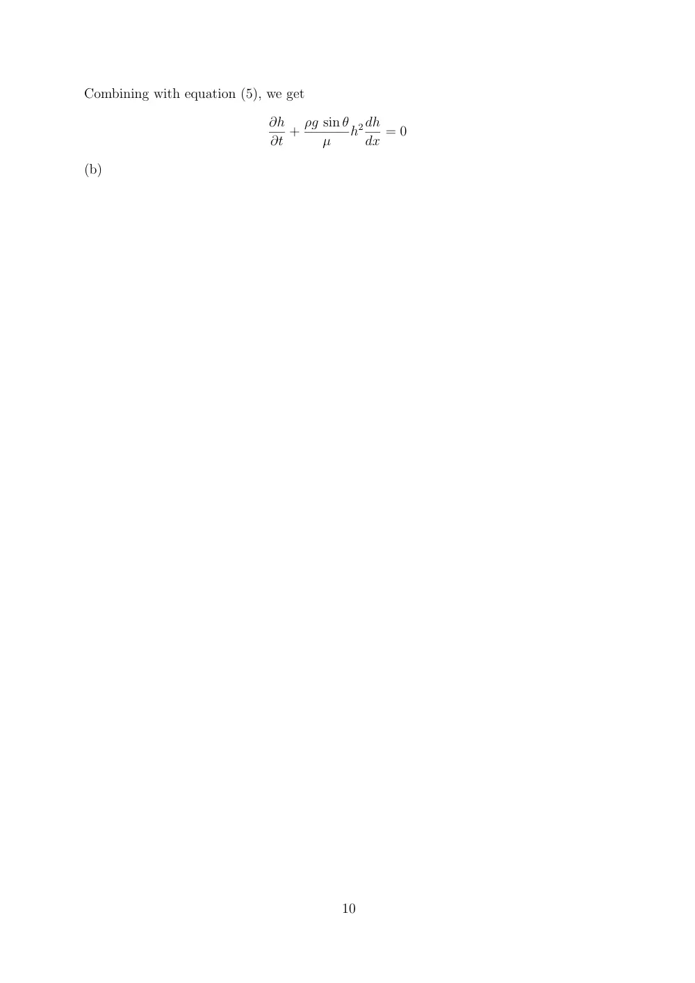The boundary conditions are u = 0 at y = 0 τ = µ∂u ∂y = 0 at y = h The velocity is then given by u = ρg sin θ µ � hy − y2 2 � The volume flow rate is Q = � h 0 u dy = ρg sin θ 3µ h3 ⇒ dQ dx = ρg sin θ µ h2dh dx 9 Combining with equation (5), we get ∂h ∂t + ρg sin θ µ h2dh dx = 0 (b) 10