MECH 314 Problems 5, Spring 2014

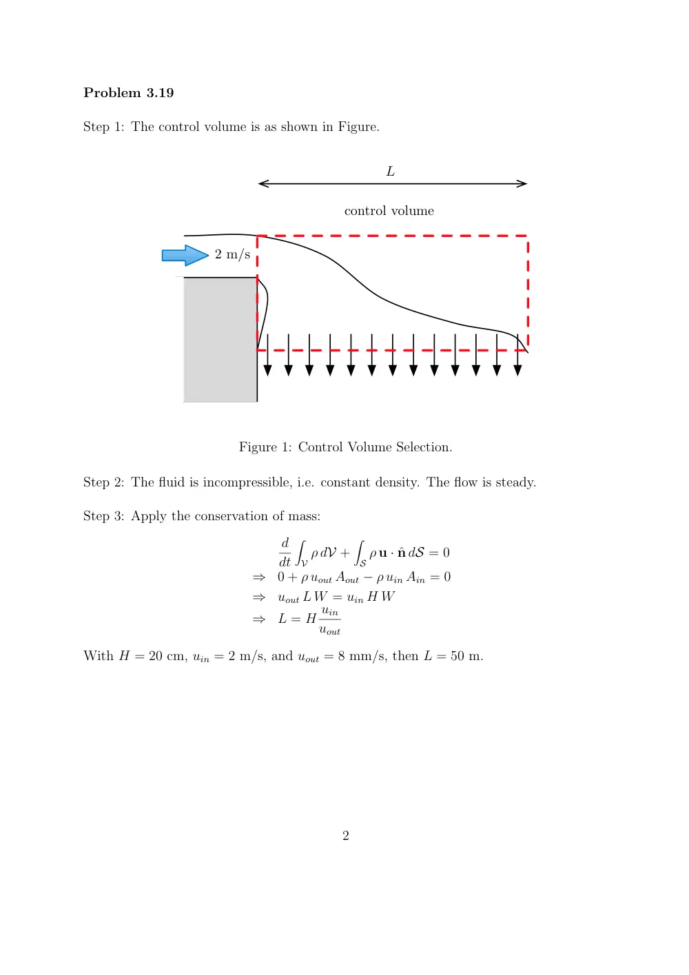
MECH 314 Introduction to Fluid Mechanics November 18, 2009 American University of Beirut, Spring 2009 Handout # PS3 Problem Set 3 Solution Textbook: Conservation of mass: Problems 3.19, 3.23, 3.25, 3.29 Conservation of momentum: Problems 3.39, 3.53, 3.80, 3.82 Conservation of energy: Problems 3.132, 3.137, 3.143, 3.144 1 Problem 3.19 Step 1: The control volume is as shown in Figure. control volume 2 m/s L Figure 1: Control Volume Selection. Step 2: The fluid is incompressible, i.e. constant density. The flow is steady. Step 3: Apply the conservation of mass: d dt � V ρ dV + � S ρ u · ˆn dS = 0 ⇒ 0 + ρ uout Aout − ρ uin Ain = 0 ⇒ uout L W = uin H W ⇒ L = H uin uout With H = 20 cm, uin = 2 m/s, and uout = 8 mm/s, then L = 50 m. 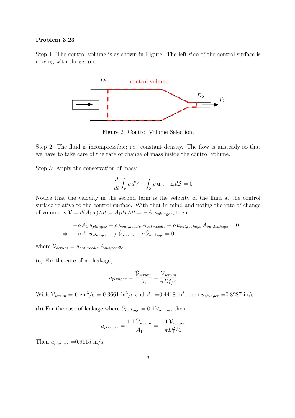2 Problem 3.23 Step 1: The control volume is as shown in Figure. The left side of the control surface is moving with the serum. D1 D2 V2 control volume Figure 2: Control Volume Selection. Step 2: The fluid is incompressible; i.e. constant density. The flow is unsteady so that we have to take care of the rate of change of mass inside the control volume. Step 3: Apply the conservation of mass: d dt � V ρ dV + � S ρ urel · ˆn dS = 0 Notice that the velocity in the second term is the velocity of the fluid at the control surface relative to the control surface. With that in mind and noting the rate of change of volume is ˙V = d(A1 x)/dt = A1dx/dt = −A1uplunger, then −ρ A1 uplunger + ρ uout,needle Aout,needle + ρ uout,leakage Aout,leakage = 0 ⇒ −ρ A1 uplunger + ρ ˙Vserum + ρ ˙Vleakage = 0 where ˙Vserum = uout,needle Aout,needle. (a) For the case of no leakage, uplunger = ˙Vserum A1 = ˙Vserum πD2 1/4 With ˙Vserum = 6 cm3/s = 0.3661 in3/s and A1 =0.4418 in2, then uplunger =0.8287 in/s. (b) For the case of leakage where ˙Vleakage = 0.1 ˙Vserum, then uplunger = 1.1 ˙Vserum A1 = 1.1 ˙Vserum πD2 1/4 Then uplunger =0.9115 in/s. 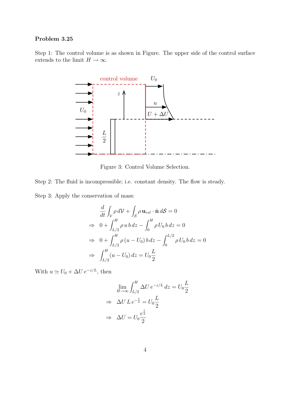3 Problem 3.25 Step 1: The control volume is as shown in Figure. The upper side of the control surface extends to the limit H → ∞. U0 U0 U + ∆U u L 2 z control volume Figure 3: Control Volume Selection. Step 2: The fluid is incompressible; i.e. constant density. The flow is steady. 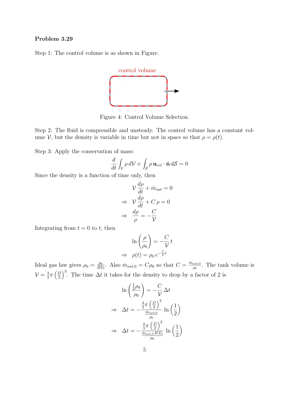Step 3: Apply the conservation of mass: d dt � V ρ dV + � S ρ urel · ˆn dS = 0 ⇒ 0 + � H L/2 ρ u b dz − � H 0 ρ U0 b dz = 0 ⇒ 0 + � H L/2 ρ (u − U0) b dz − � L/2 0 ρ U0 b dz = 0 ⇒ � H L/2(u − U0) dz = U0 L 2 With u ≃ U0 + ∆U e−z/L, then lim H→∞ � H L/2 ∆U e−z/L dz = U0 L 2 ⇒ ∆U L e− 1 2 = U0 L 2 ⇒ ∆U = U0 e 1 2 2 4 Problem 3.29 Step 1: The control volume is as shown in Figure. control volume Figure 4: Control Volume Selection. Step 2: The fluid is compressible and unsteady. The control volume has a constant vol- ume V, but the density is variable in time but not in space so that ρ = ρ(t). Step 3: Apply the conservation of mass: d dt � V ρ dV + � S ρ urel · ˆn dS = 0 Since the density is a function of time only, then V dρ dt + ˙mout = 0 ⇒ V dρ dt + C ρ = 0 ⇒ dρ ρ = −C V Integrating from t = 0 to t, then ln � ρ ρ0 � = −C V t ⇒ ρ(t) = ρ0 e− C V t Ideal gas law gives ρ0 = p0 RT0. Also ˙mout,0 = Cρ0 so that C = ˙mout,0 ρ0 . The tank volume is V = 4 3π � D 2 �3. 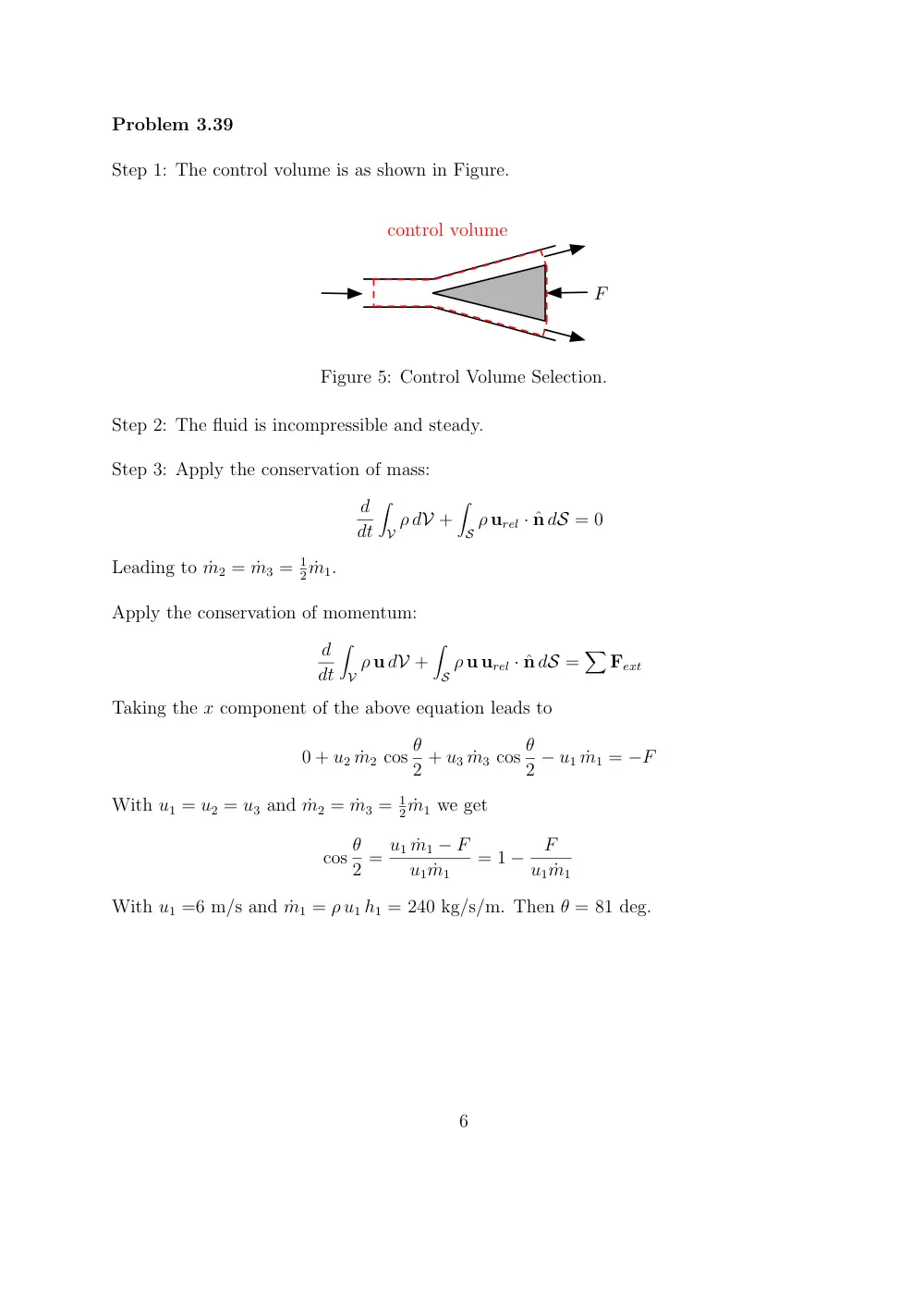The time ∆t it takes for the density to drop by a factor of 2 is ln � 1 2ρ0 ρ0 � = −C V ∆t ⇒ ∆t = − 4 3π � D 2 �3 ˙mout,0 ρ0 ln �1 2 � ⇒ ∆t = − 4 3π � D 2 �3 ˙mout,0 R T0 p0 ln �1 2 � 5 Problem 3.39 Step 1: The control volume is as shown in Figure. control volume F Figure 5: Control Volume Selection. Step 2: The fluid is incompressible and steady. Step 3: Apply the conservation of mass: d dt � V ρ dV + � S ρ urel · ˆn dS = 0 Leading to ˙m2 = ˙m3 = 1 2 ˙m1. Apply the conservation of momentum: d dt � V ρ u dV + � S ρ u urel · ˆn dS = � Fext Taking the x component of the above equation leads to 0 + u2 ˙m2 cos θ 2 + u3 ˙m3 cos θ 2 − u1 ˙m1 = −F With u1 = u2 = u3 and ˙m2 = ˙m3 = 1 2 ˙m1 we get cos θ 2 = u1 ˙m1 − F u1 ˙m1 = 1 − F u1 ˙m1 With u1 =6 m/s and ˙m1 = ρ u1 h1 = 240 kg/s/m. Then θ = 81 deg. 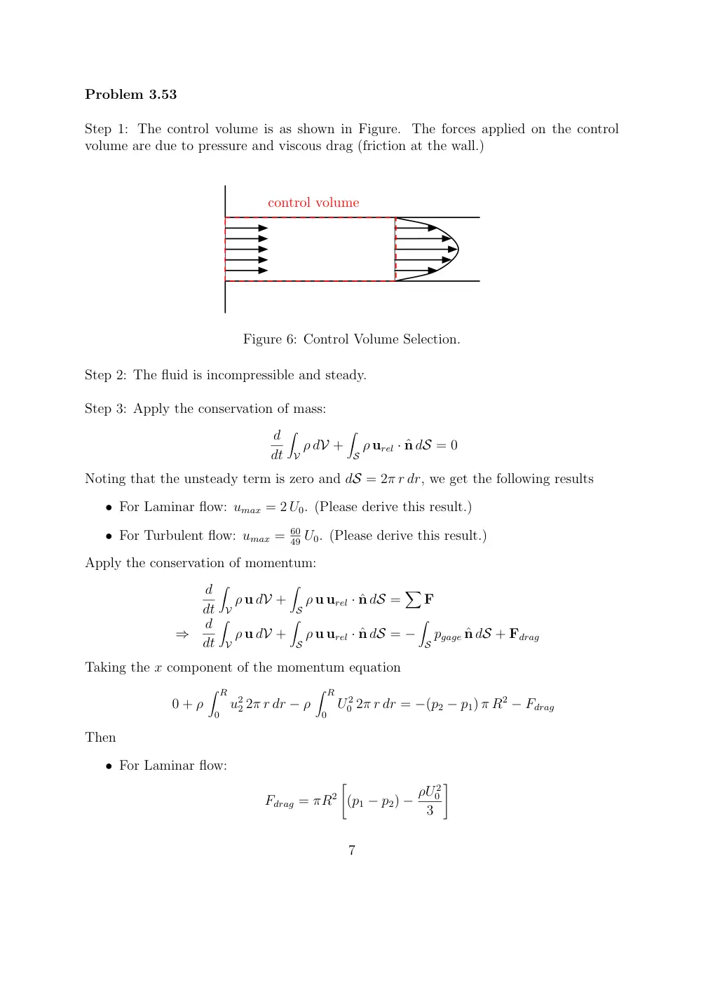6 Problem 3.53 Step 1: The control volume is as shown in Figure. The forces applied on the control volume are due to pressure and viscous drag (friction at the wall.) control volume Figure 6: Control Volume Selection. Step 2: The fluid is incompressible and steady. Step 3: Apply the conservation of mass: d dt � V ρ dV + � S ρ urel · ˆn dS = 0 Noting that the unsteady term is zero and dS = 2π r dr, we get the following results • For Laminar flow: umax = 2 U0. (Please derive this result.) • For Turbulent flow: umax = 60 49 U0. 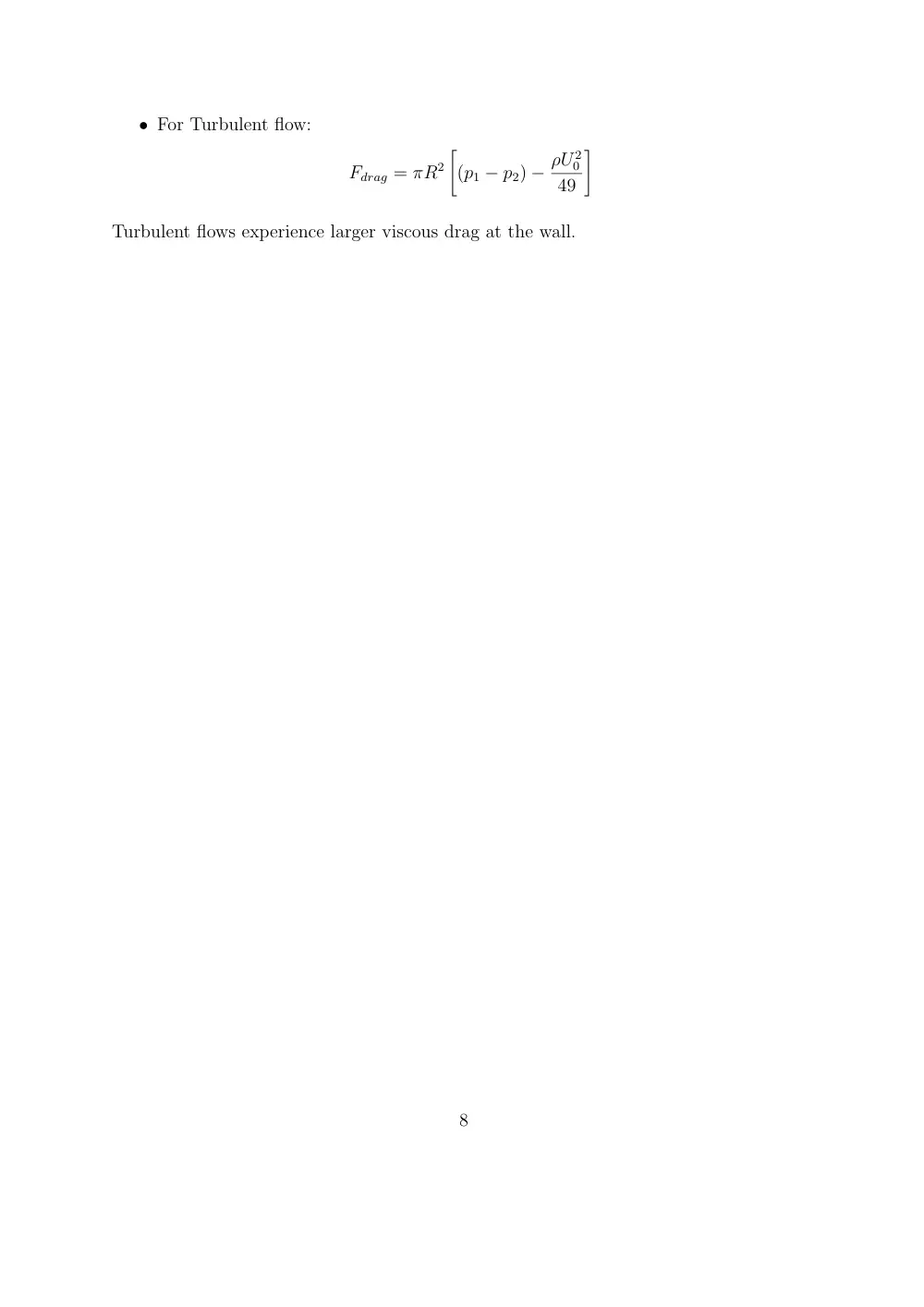(Please derive this result.) Apply the conservation of momentum: d dt � V ρ u dV + � S ρ u urel · ˆn dS = � F ⇒ d dt � V ρ u dV + � S ρ u urel · ˆn dS = − � S pgage ˆn dS + Fdrag Taking the x component of the momentum equation 0 + ρ � R 0 u2 2 2π r dr − ρ � R 0 U 2 0 2π r dr = −(p2 − p1) π R2 − Fdrag Then • For Laminar flow: Fdrag = πR2 � (p1 − p2) − ρU 2 0 3 � 7 • For Turbulent flow: Fdrag = πR2 � (p1 − p2) − ρU 2 0 49 � Turbulent flows experience larger viscous drag at the wall. 8 Problem 3.80 Step 1: The control volume is as shown in Figure. The forces applied on the control volume are due to pressure which is assumed to be hydrostatic. Viscous forces at the river bottom are neglected. control volume V1 V2 Figure 7: Control Volume Selection. Step 2: The fluid is incompressible and steady. Step 3: Apply the conservation of mass: d dt � V ρ dV + � S ρ urel · ˆn dS = 0 Noting that the unsteady term is zero then V2 = V1 h1 h2. Apply the conservation of momentum: d dt � V ρ u dV + � S ρ u urel · ˆn dS = � F ⇒ d dt � V ρ u dV + � S ρ u urel · ˆn dS = − � S pgage ˆn dS + Fviscous + Fobstacle Noting that the flow is steady and the viscous drag is neglected and that the velocity at sections 1 and 2 is uniform. Taking the x component of the momentum equation 0 + ˙m V2 − ˙m V1 = − � h2 0 p2,gage b dz + � h1 0 p1,gage b dz − Fobstacle Note that if the flow exerts a force Fobstacle on the obstacle, then the obstacle exerts a force of −Fobstacle on the fluid. 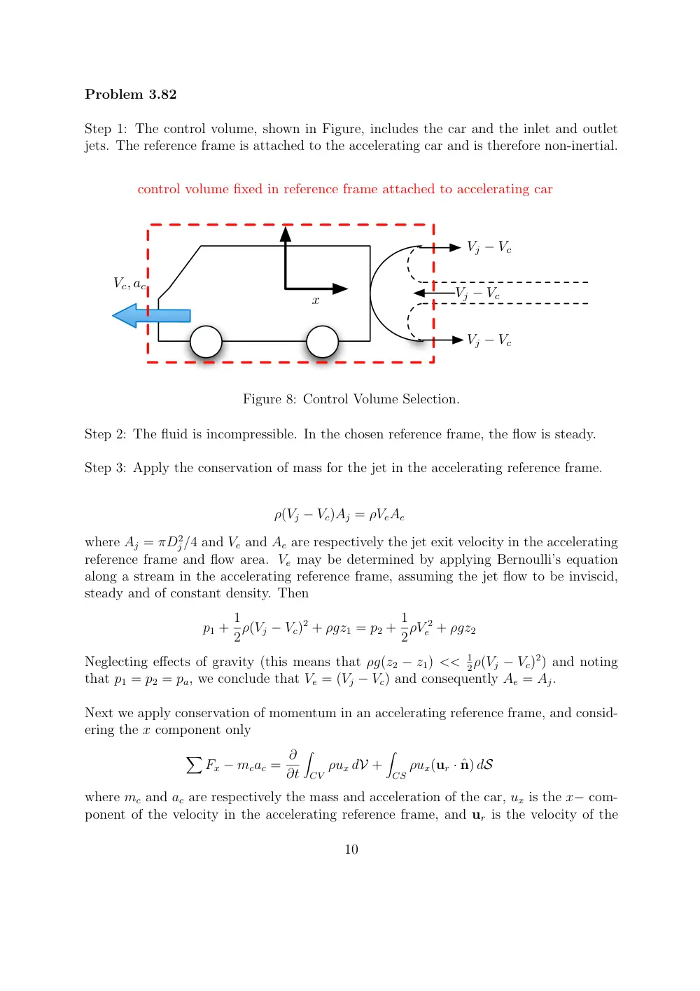Noting that the hydrostatic pressure is p1,gage = ρ g (h1 −z) and p2,gage = ρ g (h2 − z), then Fobstacle = ˙m (V1 − V2) + ρ g b 2 � h2 1 − h2 2 � = ρ V1 b h1 � V1 − V1 h1 h2 � + ρ g b 2 � h2 1 − h2 2 � = −ρ V 2 1 b h1 �h1 h2 − 1 � + ρ g b 2 � h2 1 − h2 2 � 9 Problem 3.82 Step 1: The control volume, shown in Figure, includes the car and the inlet and outlet jets. The reference frame is attached to the accelerating car and is therefore non-inertial. Vc, ac x control volume fixed in reference frame attached to accelerating car Vj − Vc Vj − Vc Vj − Vc Figure 8: Control Volume Selection. Step 2: The fluid is incompressible. In the chosen reference frame, the flow is steady. Step 3: Apply the conservation of mass for the jet in the accelerating reference frame. ρ(Vj − Vc)Aj = ρVeAe where Aj = πD2 j/4 and Ve and Ae are respectively the jet exit velocity in the accelerating reference frame and flow area. Ve may be determined by applying Bernoulli’s equation along a stream in the accelerating reference frame, assuming the jet flow to be inviscid, steady and of constant density. Then p1 + 1 2ρ(Vj − Vc)2 + ρgz1 = p2 + 1 2ρV 2 e + ρgz2 Neglecting effects of gravity (this means that ρg(z2 − z1) << 1 2ρ(Vj − Vc)2) and noting that p1 = p2 = pa, we conclude that Ve = (Vj − Vc) and consequently Ae = Aj. Next we apply conservation of momentum in an accelerating reference frame, and consid- ering the x component only � Fx − mcac = ∂ ∂t � CV ρux dV + � CS ρux(ur · ˆn) dS where mc and ac are respectively the mass and acceleration of the car, ux is the x− com- ponent of the velocity in the accelerating reference frame, and ur is the velocity of the 10 flow with respect to the control surface. Since the flow is steady in the car reference frame, and the forces due to air drag and wheel friction with ground are neglected, then −mcac = � CS ρux(ur · ˆn) dS Noting that � CS ρ(ur · ˆn) dS = −ρ(Vj − Vc)Aj for the inlet flow and ρ(Vj − Vc)Aj for the outlet flow, where Vj − Vc is the speed of the jet relative to the car moving at Vc. And noting that ux = −(Vj − Vc) for the inlet flow and (Vj − Vc) for the outlet flow, then −mcac = 2ρ(Vj − Vc)2Aj It is important to note the pressure is atmospheric throughout the control surface. In particular, the pressure across a free straight jet characterized by large Reynolds number Re = ρVjDj/µ >> 1 is atmospheric. This, along with Bernoulli’s equation, will be ex- plained and discussed further when we study inviscid flows. Another important thing to look at is applying the conservation of mass for the jet by taking a fixed control mass with its right side fixed at the jet exit from the nozzle and its left side moving with the car. How will the conservation of mass look like? Can we neglect the transient term in this case? 11