PHY 201 Chapter 23, Fall 2017

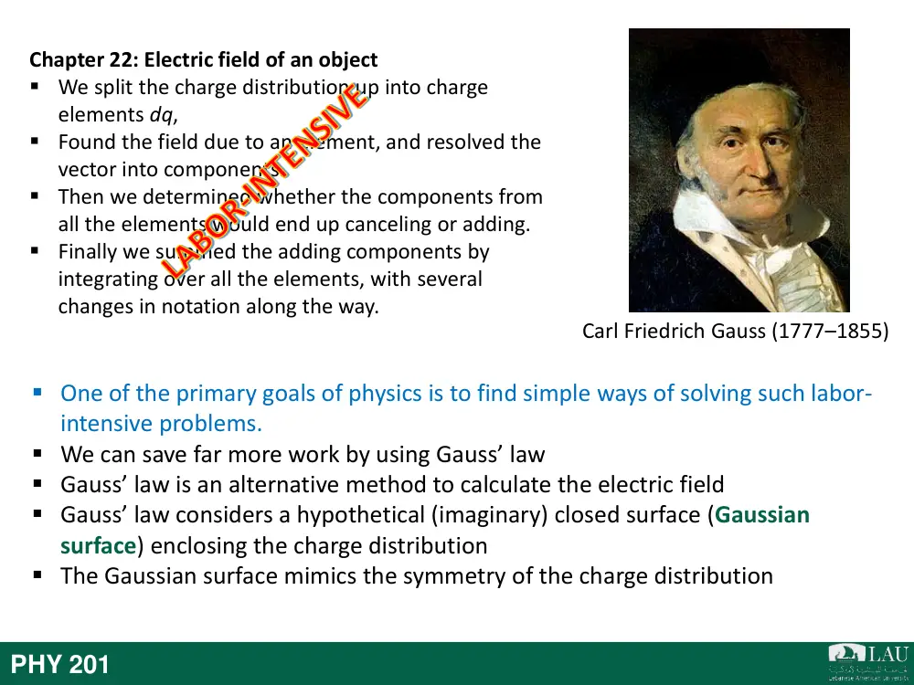
CHAPTER 23 GAUSS’ LAW INTRODUCTION 23-1 PHY 201 Carl Friedrich Gauss (1777–1855) Chapter 22: Electric field of an object  We split the charge distribution up into charge elements dq,  Found the field due to an element, and resolved the vector into components.  Then we determined whether the components from all the elements would end up canceling or adding.  Finally we summed the adding components by integrating over all the elements, with several changes in notation along the way.  One of the primary goals of physics is to find simple ways of solving such labor- intensive problems.  We can save far more work by using Gauss’ law  Gauss’ law is an alternative method to calculate the electric field  Gauss’ law considers a hypothetical (imaginary) closed surface (Gaussian surface) enclosing the charge distribution  The Gaussian surface mimics the symmetry of the charge distribution PHY 201 The problems in this chapter are of two types: - Sometimes we know the charge and we use Gauss’ law to find the field at some point. - Sometimes we know the field on a Gaussian surface and we use Gauss’ law to find the charge enclosed by the surface. We need a quantitative way of determining how much electric field pierces a surface. That measure is called the electric flux. 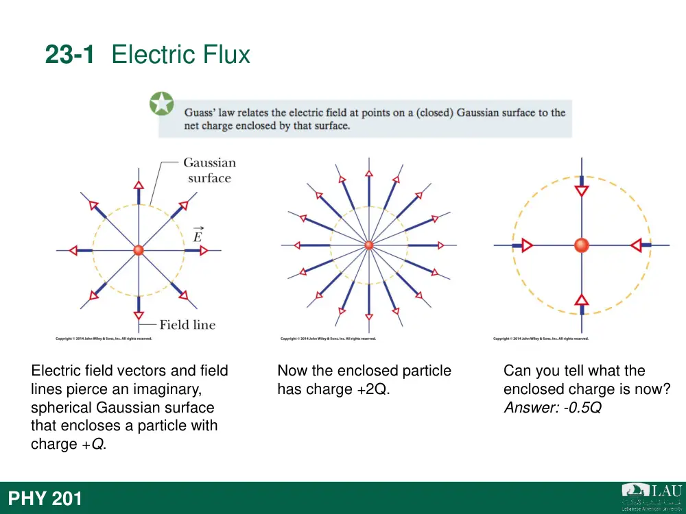Electric Flux 23-1 PHY 201 23-1 Electric Flux Electric field vectors and field lines pierce an imaginary, spherical Gaussian surface that encloses a particle with charge +Q. Now the enclosed particle has charge +2Q. Can you tell what the enclosed charge is now? 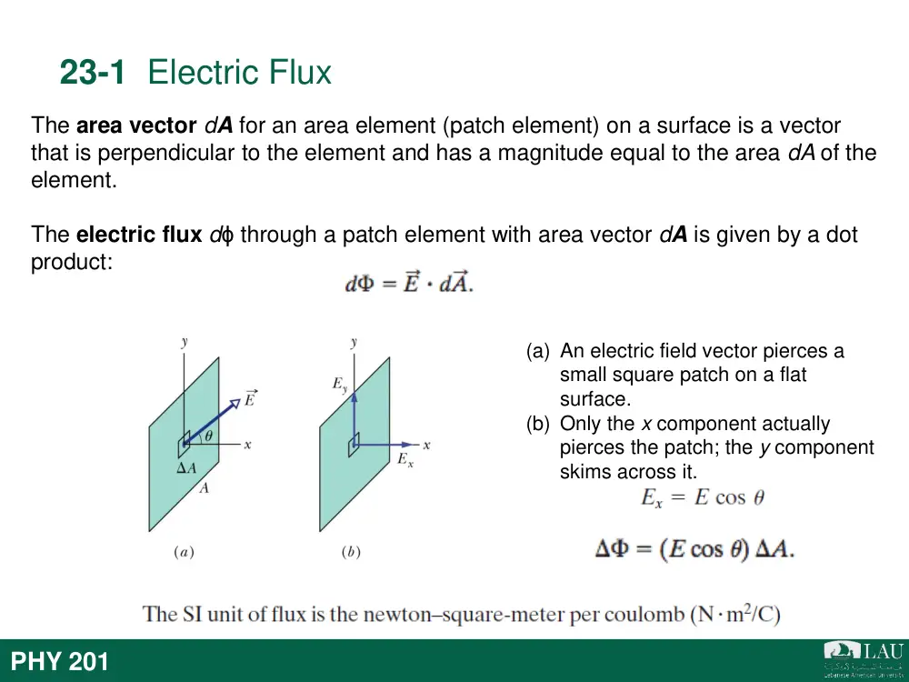Answer: -0.5Q PHY 201 The area vector dA for an area element (patch element) on a surface is a vector that is perpendicular to the element and has a magnitude equal to the area dA of the element. The electric flux dϕ through a patch element with area vector dA is given by a dot product: (a) An electric field vector pierces a small square patch on a flat surface. (b) Only the x component actually pierces the patch; the y component skims across it. 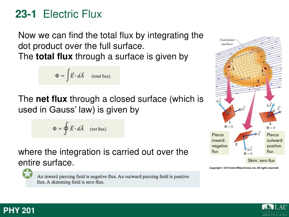23-1 Electric Flux PHY 201 Now we can find the total flux by integrating the dot product over the full surface. The total flux through a surface is given by The net flux through a closed surface (which is used in Gauss’ law) is given by where the integration is carried out over the entire surface. 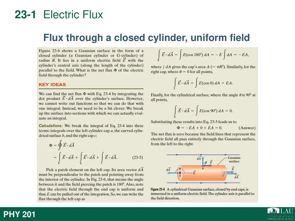23-1 Electric Flux PHY 201 23-1 Electric Flux Flux through a closed cylinder, uniform field GAUSS’ LAW 23-2 PHY 201 23-2 Gauss’ Law Gauss’ law relates the net flux ϕ of an electric field through a closed surface (a Gaussian surface) to the net charge qenc that is enclosed by that surface. It tells us that we can also write Gauss’ law as PHY 201 23-2 Gauss’ Law Surface S1.The electric field is outward for all points on this surface. Thus, the flux of the electric field through this surface is positive, and so is the net charge within the surface, as Gauss’ law requires Surface S2.The electric field is inward for all points on this surface. Thus, the flux of the electric field through this surface is negative and so is the enclosed charge, as Gauss’ law requires. Two charges, equal in magnitude but opposite in sign, and the field lines that represent their net electric field. Four Gaussian surfaces are shown in cross section. PHY 201 23-2 Gauss’ Law Surface S3.This surface encloses no charge, and thus qenc = 0. Gauss’ law requires that the net flux of the electric field through this surface be zero. That is reasonable because all the field lines pass entirely through the surface, entering it at the top and leaving at the bottom. Surface S4.This surface encloses no net charge, because the enclosed positive and negative charges have equal magnitudes. Gauss’ law requires that the net flux of the electric field through this surface be zero. That is reasonable because there are as many field lines leaving surface S4 as entering it. Two charges, equal in magnitude but opposite in sign, and the field lines that represent their net electric field. Four Gaussian surfaces are shown in cross section. A Charged Isolated Conductor 23-3 PHY 201 23-3 A Charged Isolated Conductor + + + + + + + + + +  The electric field inside a conductor is zero  Gauss’ law is used to find the electric field magnitude E near an isolated conducting surface with a uniform surface charge density σ. PHY 201 (a) Perspective view (b) Side view of a tiny portion of a large, isolated conductor with excess positive charge on its surface. A (closed) cylindrical Gaussian surface, embedded perpendicularly in the conductor, encloses some of the charge. Electric field lines pierce the external end cap of the cylinder, but not the internal end cap. The external end cap has area A and area vector A. 23-3 A Charged Isolated Conductor Applying Gauss’ Law: Cylindrical Symmetry 23-4 PHY 201 23-4 Applying Gauss’ Law: Cylindrical Symmetry Figure shows a section of an infinitely long cylindrical plastic rod with a uniform charge density λ. The charge distribution and the field have cylindrical symmetry. To find the field at radius r, we enclose a section of the rod with a concentric Gaussian cylinder of radius r and height h. The net flux through the cylinder from Gauss’ Law reduces to yielding A Gaussian surface in the form of a closed cylinder surrounds a section of a very long, uniformly charged, cylindrical plastic rod. Applying Gauss’ Law: Planar Symmetry 23-5 PHY 201 23-5 Applying Gauss’ Law: Planar Symmetry Figure (a-b) shows a portion of a thin, infinite, non- conducting sheet with a uniform (positive) surface charge density σ. A sheet of thin plastic wrap, uniformly charged on one side, can serve as a simple model. Gauss’ Law, becomes where σA is the charge enclosed by the Gaussian surface. This gives Non-conducting thin Sheet PHY 201 23-5 Applying Gauss’ Law: Planar Symmetry Figure (a) shows a cross section of a thin, infinite conducting plate with excess positive charge. Figure (b) shows an identical plate with excess negative charge having the same magnitude of surface charge density σ1. Suppose we arrange for the plates of Figs. a and b to be close to each other and parallel (c). Since the plates are conductors, when we bring them into this arrangement, the excess charge on one plate attracts the excess charge Two conducting Plates on the other plate, and all the excess charge moves onto the inner faces of the plates as in Fig.c. With twice as much charge now on each inner face, the electric field at any point between the plates has the magnitude 23-6 Applying Gauss’ Law: Spherical Symmetry PHY 201 23-6 Applying Gauss’ Law: Spherical Symmetry A thin, uniformly charged, spherical shell with total charge q, in cross section. Two Gaussian surfaces S1 and S2 are also shown in cross section. Surface S2 encloses the shell, and S1 encloses only the empty interior of the shell. In the figure, applying Gauss’ law to surface S2, for which r ≥ R, we would find that And, applying Gauss’ law to surface S1, for which r < R, PHY 201 23-6 Applying Gauss’ Law: Spherical Symmetry Inside a sphere with a uniform volume charge density, the field is radial and has the magnitude where q is the total charge, R is the sphere’s radius, and r is the radial distance from the center of the sphere to the point of measurement as shown in figure. A concentric spherical Gaussian surface with r > R is shown in (a). A similar Gaussian surface with r < R is shown in (b). 23-4 SUMMARY PHY 201 23 Summary Gauss’ Law • Gauss’ law is • the net flux of the electric field through the surface: • Infinite non-conducting sheet • Outside a spherical shell of charge • Inside a uniform spherical shell • Inside a uniform sphere of charge Eq. 23-15 Eq. 23-20 Applications of Gauss’ Law • surface of a charged conductor • Within the surface E=0. • line of charge Eq. 23-6 Eq. 23-11 Eq. 23-6 Eq. 23-12 Eq. 23-13 Eq. 23-16