PHY 201 Chapter 30, Fall 2017

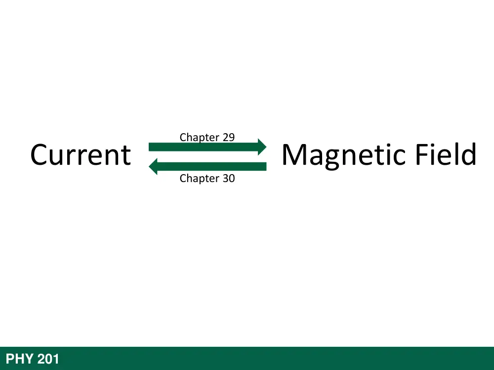
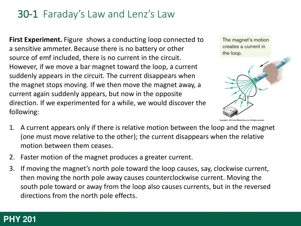
CHAPTER 30 Induction and Inductance 30-1 Faraday’s Law and Lenz’s Law PHY 201 Current Magnetic Field Chapter 29 Chapter 30 30-1 Faraday’s Law and Lenz’s Law First Experiment. Figure shows a conducting loop connected to a sensitive ammeter. Because there is no battery or other source of emf included, there is no current in the circuit. However, if we move a bar magnet toward the loop, a current suddenly appears in the circuit. The current disappears when the magnet stops moving. If we then move the magnet away, a current again suddenly appears, but now in the opposite direction. If we experimented for a while, we would discover the following: 1. A current appears only if there is relative motion between the loop and the magnet (one must move relative to the other); the current disappears when the relative motion between them ceases. 2. Faster motion of the magnet produces a greater current. 3. If moving the magnet’s north pole toward the loop causes, say, clockwise current, then moving the north pole away causes counterclockwise current. Moving the south pole toward or away from the loop also causes currents, but in the reversed directions from the north pole effects. 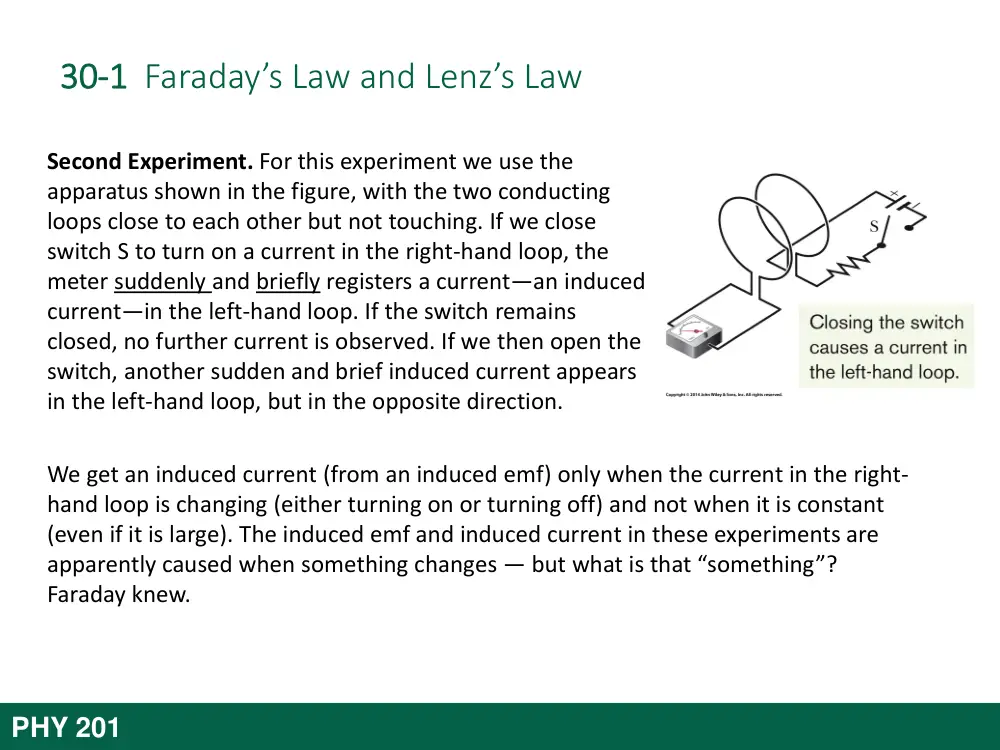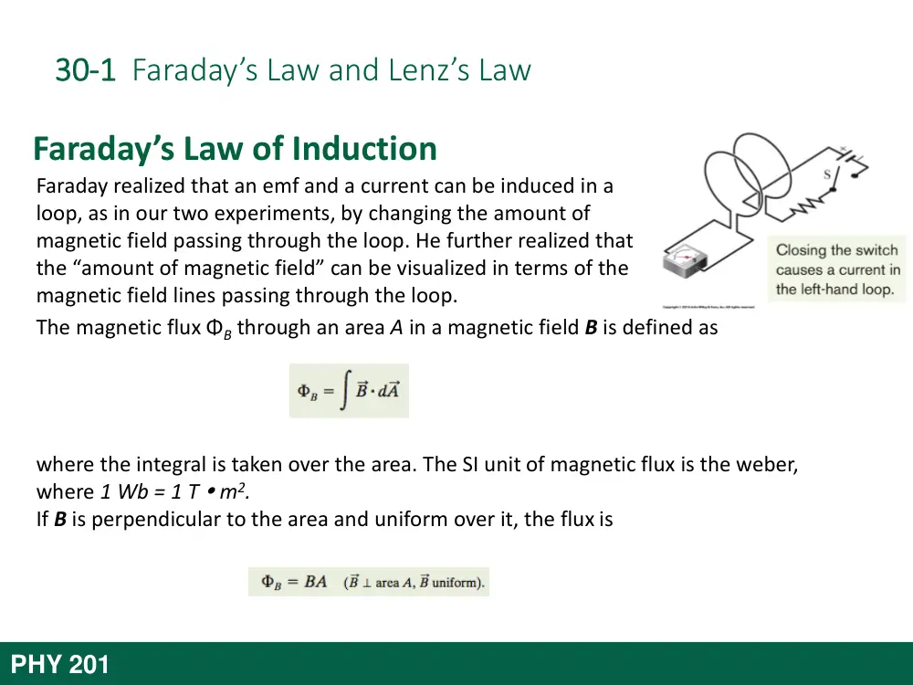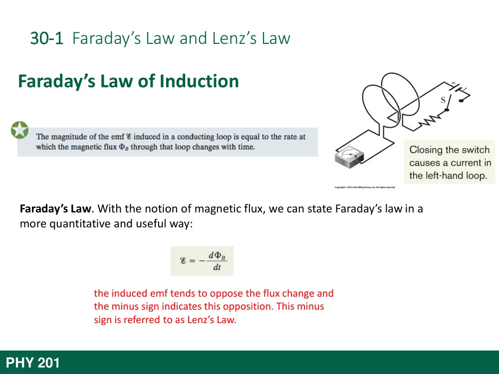PHY 201 30-1 Faraday’s Law and Lenz’s Law Second Experiment. For this experiment we use the apparatus shown in the figure, with the two conducting loops close to each other but not touching. If we close switch S to turn on a current in the right-hand loop, the meter suddenly and briefly registers a current—an induced current—in the left-hand loop. If the switch remains closed, no further current is observed. If we then open the switch, another sudden and brief induced current appears in the left-hand loop, but in the opposite direction. We get an induced current (from an induced emf) only when the current in the right- hand loop is changing (either turning on or turning off) and not when it is constant (even if it is large). The induced emf and induced current in these experiments are apparently caused when something changes — but what is that “something”? Faraday knew. 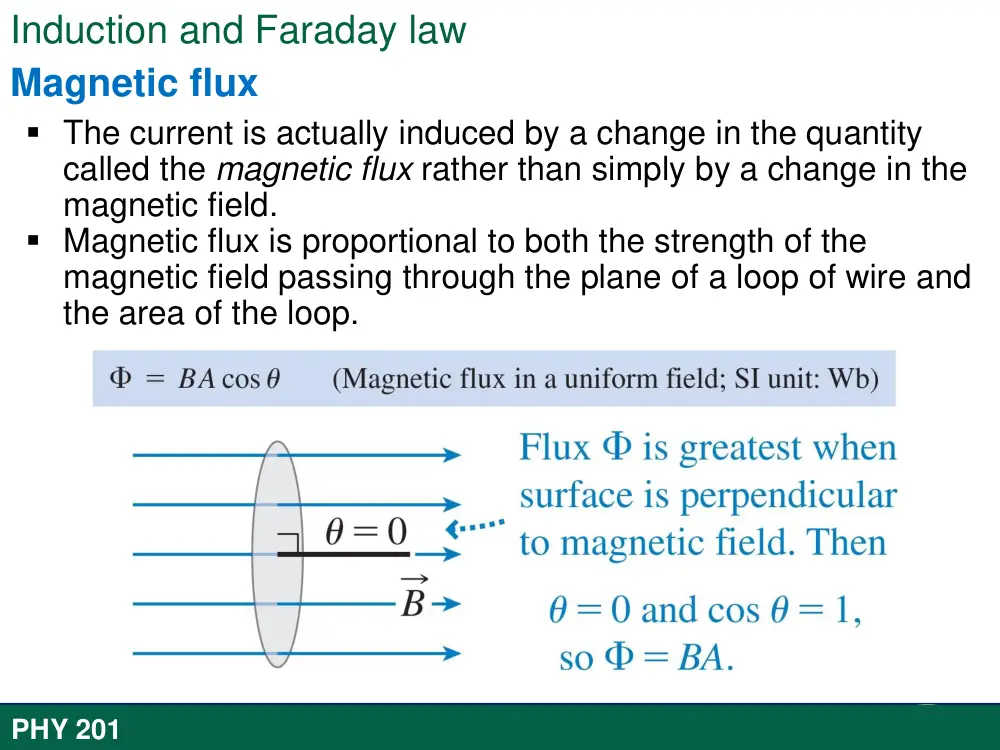PHY 201 PHY 305 Induction and Faraday law Magnetic flux  The current is actually induced by a change in the quantity called the magnetic flux rather than simply by a change in the magnetic field.  Magnetic flux is proportional to both the strength of the magnetic field passing through the plane of a loop of wire and the area of the loop. 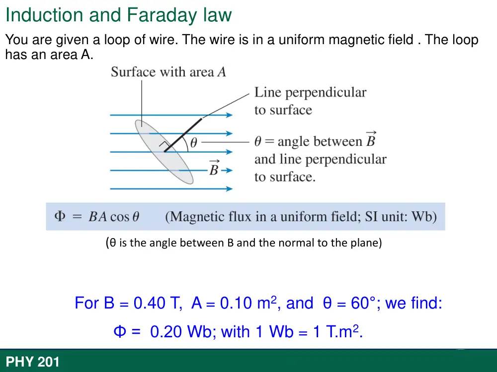PHY 201 PHY 305 Induction and Faraday law You are given a loop of wire. The wire is in a uniform magnetic field . The loop has an area A. (θ is the angle between B and the normal to the plane) For B = 0.40 T, A = 0.10 m2, and θ = 60°; we find: Φ = 0.20 Wb; with 1 Wb = 1 T.m2. 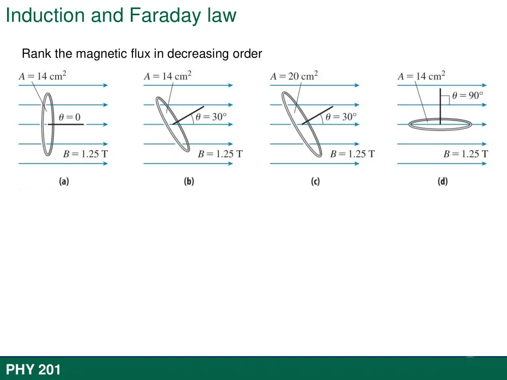PHY 201 PHY 305 Induction and Faraday law Rank the magnetic flux in decreasing order PHY 201 30-1 Faraday’s Law and Lenz’s Law The magnetic flux ΦB through an area A in a magnetic field B is defined as where the integral is taken over the area. The SI unit of magnetic flux is the weber, where 1 Wb = 1 T  m2. If B is perpendicular to the area and uniform over it, the flux is Faraday’s Law of Induction Faraday realized that an emf and a current can be induced in a loop, as in our two experiments, by changing the amount of magnetic field passing through the loop. He further realized that the “amount of magnetic field” can be visualized in terms of the magnetic field lines passing through the loop. PHY 201 30-1 Faraday’s Law and Lenz’s Law Faraday’s Law. With the notion of magnetic flux, we can state Faraday’s law in a more quantitative and useful way: Faraday’s Law of Induction the induced emf tends to oppose the flux change and the minus sign indicates this opposition. This minus sign is referred to as Lenz’s Law. PHY 201 30-1 Faraday’s Law and Lenz’s Law Lenz’s Law An induced current has a direction such that the magnetic field due to this induced current opposes the change in the magnetic flux that induces the current. The induced emf has the same direction as the induced current. Lenz’s law at work. As the magnet is moved toward the loop, a current is induced in the loop. The current produces its own magnetic field, with magnetic dipole moment μ oriented so as to oppose the motion of the magnet. Thus, the induced current must be counterclockwise as shown. PHY 201 PHY 305 Induction and Faraday law ΦB B and Bin have opposite directions ΦB B and Bin have same direction When applying Lenz’ Law, there are two magnetic fields to consider: - B: The external changing magnetic field - B induced: The magnetic field produced by the current in the loop. PHY 201 30-1 Faraday’s Law and Lenz’s Law Lenz’s Law The direction of the current i induced in a loop is such that the current’s magnetic field Bind opposes the change in the magnetic field B inducing i. The field Bind is always directed opposite an increasing field B (a, c) and in the same direction as a decreasing field B (b, d ). The curled – straight right-hand rule gives the direction of the induced current based on the direction of the induced field. PHY 201 PHY 305 Induction and Faraday law Find the direction of the induced current in each. PHY 201 30-2 Induction and Energy Transfer 30-2 Induction and Energy Transfer In the figure, a rectangular loop of wire of width L has one end in a uniform external magnetic field that is directed perpendicularly into the plane of the loop. This field may be produced, for example, by a large electromagnet. The dashed lines in the figure show the assumed limits of the magnetic field; the fringing of the field at its edges is neglected. You are to pull this loop to the right at a constant velocity v. Flux change: Therefore, in the figure a magnetic field and a conducting loop are in relative motion at speed v and the flux of the field through the loop is changing with time (here the flux is changing as the area of the loop still in the magnetic field is changing). Rate of Work: To pull the loop at a constant velocity v, you must apply a constant force F to the loop because a magnetic force of equal magnitude but opposite direction acts on the loop to oppose you. The rate at which you do work — that is, the power — is then where F is the magnitude of the force you apply to the loop. PHY 201 30-2 Induction and Energy Transfer Induced emf: To find the current, we first apply Faraday’s law. When x is the length of the loop still in the magnetic field, the area of the loop still in the field is Lx. Then, the magnitude of the flux through the loop is As x decreases, the flux decreases. Faraday’s law tells us that with this flux i decrease, an emf is induced in the loop. We can write the magnitude of this emf as in which we have replaced dx/dt with v, the speed at which the loop moves. A circuit diagram for the loop of above figure while the loop is moving. PHY 201 30-2 Induction and Energy Transfer Induced Current: Figure (bottom) shows the loop as a circuit: induced emf is represented on the left, and the collective resistance R of the loop is represented on the right. To find the magnitude of the induced current, we can apply the equation which gives In the Fig. (top), the deflecting forces acting on the three segments of the loop are marked F1, F2, and F3. Note, however, that from the symmetry, forces F2 and F3 are equal in magnitude and cancel. This leaves only force F1, which is directed opposite your force F on the loop and thus is the force opposing you. A circuit diagram for the loop of above figure while the loop is moving. PHY 201 30-2 Induction and Energy Transfer So, F = -F1. the magnitude of F1 thus where the angle between B and the length vector L for the left segment is 90°. This gives us Because B, L, and R are constants, the speed v at which you move the loop is constant if the magnitude F of the force you apply to the loop is also constant. Rate of Work: We find the rate at which you do work on the loop as you pull it from the magnetic field: NOTE: The work that you do in pulling the loop through the magnetic field appears as thermal energy in the loop. A circuit diagram for the loop of above figure while the loop is moving. PHY 201 30-4 Inductors and Inductance 30-4 Inductors and Inductance The crude inductors with which Michael Faraday discovered the law of induction. In those days amenities such as insulated wire were not commercially available. It is said that Faraday insulated his wires by wrapping them with strips cut from one of his wife’s petticoats. An inductor is a device that can be used to produce a known magnetic field in a specified region. If a current i is established through each of the N windings of an inductor, a magnetic flux ΦB links those windings. The inductance L of the inductor is The SI unit of inductance is the henry (H), where 1 henry = 1H=1Tm2/A. The inductance per unit length near the middle of a long solenoid of cross-sectional area A and n turns per unit length is PHY 201 30-5 Self-Induction 30-5 Self-Induction If two coils — which we can now call inductors — are near each other, a current i in one coil produces a magnetic flux ΦB through the second coil. We have seen that if we change this flux by changing the current, an induced emf appears in the second coil according to Faraday’s law. An induced emf appears in the first coil as well. This process (see Figure) is called self-induction, and the emf that appears is called a self-induced emf. It obeys Faraday’s law of induction just as other induced emfs do. For any inductor, Faraday’s law tells us that By combining these equations, we can write Note: Thus, in any inductor (such as a coil, a solenoid, or a toroid) a self- induced emf appears whenever the current changes with time. The magnitude of the current has no influence on the magnitude of the induced emf; only the rate of change of the current counts. PHY 201 30-6 RL Circuits PHY 201 A first order non-homogeneous differential equation: 𝑎 𝑑𝑖(𝑡) 𝑑𝑡 + 𝑏𝑖 𝑡 + 𝑐 = 0 where a,b,c are constants General solution: i 𝑡 = 𝐾𝑒−𝑏 𝑎𝑡 + 𝑐 𝑏 [𝑒−𝑏 𝑎𝑡 − 1] 𝑖 𝑡 = ℰ 𝑅 [1 − 𝑒−𝑅 𝐿𝑡] i 𝑡 = ℰ 𝑅 𝑒−𝑅 𝐿𝑡 30-6 RL Circuits If a constant emf is introduced into a single-loop circuit containing a resistance R and an inductance L, the current rises to an equilibrium value of /R according to Here τL, the inductive time constant, is given by An RL circuit. Plot (a) and (b) shows how the potential differences VR (= iR) across the resistor and VL (= L di/dt) across the inductor vary with time for particular values of , L, and R. When the source of constant emf is removed and replaced by a conductor, the current decays from a value i0 according to The variation with time of (a) VR, the potential difference across the resistor in the circuit (top), and (b) VL, the potential difference across the inductor in that circuit. PHY 201 30-7 Energy Stored in a Magnetic Field 30-7 Energy Stored in a Magnetic Field An RL circuit. If an inductor L carries a current i, the inductor’s magnetic field stores an energy given by PHY 201 30-8 Mutual inductance 30-8 Mutual Induction If coils 1 and 2 are near each other, a changing current in either coil can induce an emf in the other. This mutual induction is described by and Mutual induction. (a) The magnetic field B1 produced by current i1 in coil 1 extends through coil 2. If i1 is varied (by varying resistance R), an emf is induced in coil 2 and current registers on the meter connected to coil 2. (b) The roles of the coils interchanged. PHY 201 CHAPTER 31 Electromagnetic Oscillations and Alternating Current 31-1 Electromagnetic Oscillations 31-1 Electromagnetic Oscillations Eight stages in a single cycle of oscillation of a resistance less LC circuit. The bar graphs by each figure show the stored magnetic and electrical energies. The magnetic field lines of the inductor and the electric field lines of the capacitor are shown. (a) Capacitor with maximum charge, no current. (b) Capacitor discharging, current increasing. (c) Capacitor fully discharged, current maximum. (d) Capacitor charging but with polarity opposite that in (a), current decreasing. (e) Capacitor with maximum charge having polarity opposite that in (a), no current. ( f ) Capacitor discharging, current increasing with direction opposite that in (b). (g) Capacitor fully discharged, current maximum. (h) Capacitor charging, current decreasing. PHY 201 31-1 Electromagnetic Oscillations Parts (a) through (h) of the Figure show succeeding stages of the oscillations in a simple LC circuit. The energy stored in the electric field of the capacitor at any time is where q is the charge on the capacitor at that time. The energy stored in the magnetic field of the inductor at any time is where i is the current through the inductor at that time. The resulting oscillations of the capacitor’s electric field and the inductor’s magnetic field are said to be electromagnetic oscillations. PHY 201 PHY 201 31-1 Electromagnetic Oscillations From the table we can deduce the correspondence between these systems. Thus, q corresponds to x, 1/C corresponds to k, i corresponds to v, and L corresponds to m. The correspondences listed above suggest that to find the angular frequency of oscillation for an ideal (resistanceless) LC circuit, k should be replaced by 1/C and m by L, yielding PHY 201 31-1 Electromagnetic Oscillations LC Oscillator The total energy U present at any instant in an oscillating LC circuit is given by in which UB is the energy stored in the magnetic field of the inductor and UE is the energy stored in the electric field of the capacitor. Since we have assumed the circuit resistance to be zero, no energy is transferred to thermal energy and U remains constant with time. In more formal language, dU/dt must be zero. This leads to However, i = dq/dt and di/dt = d2q/dt2. With these substitutions, we get This is the differential equation that describes the oscillations of a resistanceless LC circuit. PHY 201 31-1 Electromagnetic Oscillations Charge and Current Oscillation The solution for the differential equation equation that describes the oscillations of a resistanceless LC circuit is where Q is the amplitude of the charge variations, ω is the angular frequency of the electromagnetic oscillations, and ϕ is the phase constant. Taking the first derivative of the above Eq. with respect to time gives us the current: Answer: (a) εL= 12 V (b) UB=150 μJ PHY 201 31-1 Electromagnetic Oscillations Electrical and Magnetic Energy Oscillations The electrical energy stored in the LC circuit at time t is, The magnetic energy is, Figure shows plots of UE (t) and UB (t) for the case of ϕ=0. Note that 1. The maximum values of UE and UB are both Q2/2C. 2. At any instant the sum of UE and UB is equal to Q2/2C, a constant. 3. When UE is maximum, UB is zero, and conversely. The stored magnetic energy and electrical energy in the RL circuit as a function of time. PHY 201 31-2 Damped Oscillation in an RLC circuit 31-2 Damped Oscillation in an RLC circuit A series RLC circuit. As the charge contained in the circuit oscillates back and forth through the resistance, electromagnetic energy is dissipated as thermal energy, damping (decreasing the amplitude of) the oscillations. To analyze the oscillations of this circuit, we write an equation for the total electromagnetic energy U in the circuit at any instant. Because the resistance does not store electromagnetic energy, we can write Now, however, this total energy decreases as energy is transferred to thermal energy. The rate of that transfer is, where the minus sign indicates that U decreases. By differentiating U with respect to time and then substituting the result we eventually get, which is the differential equation for damped oscillations in an RLC circuit. Charge Decay. The solution to above Eq. is in which and . PHY 201 31-3 Forced Oscillations of Three Simple Circuits 31-3 Forced Oscillations of Three Simple Circuits Forced Oscillations PHY 201 31-3 Forced Oscillations of Three Simple Circuits Resistive Load The alternating potential difference across a resistor has amplitude where VR and IR are the amplitudes of alternating current iR and alternating potential difference vr across the resistance in the circuit. Angular speed: Both current and potential difference phasors rotate counterclockwise about the origin with an angular speed equal to the angular frequency ωd of vR and iR. Length: The length of each phasor represents the amplitude of the alternating quantity: VR for the voltage and IR for the current. Projection: The projection of each phasor on the vertical axis represents the value of the alternating quantity at time t: vR for the voltage and iR for the current. Rotation angle: The rotation angle of each phasor is equal to the phase of the alternating quantity at time t. A resistor is connected across an alternating-current generator. (a) The current iR and the potential difference vR across the resistor are plotted on the same graph, both versus time t. They are in phase and complete one cycle in one period T. (b) A phasor diagram shows the same thing as (a). PHY 201 31-3 Forced Oscillations of Three Simple Circuits Inductive Load The inductive reactance of an inductor is defined as Its value depends not only on the inductance but also on the driving angular frequency ωd. The voltage amplitude and current amplitude are related by Fig. (left), shows that the quantities iL and vL are 90° out of phase. In this case, however, iL lags vL; that is, monitoring the current iL and the potential difference vL in the circuit of Fig. (top) shows that iL reaches its maximum value after vL does, by one-quarter cycle. PHY 201 An inductor is connected across an alternating- current generator. 31-3 Forced Oscillations of Three Simple Circuits Capacitive Load The capacitive reactance of a capacitor, defined as Its value depends not only on the capacitance but also on the driving angular frequency ωd. The voltage amplitude and current amplitude are related by In the phasor diagram we see that iC leads vC, which means that, if you monitored the current iC and the potential difference vC in the circuit above, you would find that iC reaches its maximum before vC does, by one-quarter cycle. PHY 201 A capacitor is connected across an alternating- current generator. 31-4 The Series RLC Circuits 31-4 The Series RLC Circuit Series RLC circuit with an external emf For a series RLC circuit with an external emf given by The current is given by the current amplitude is given by The denominator in the above equation is called the impedance Z of the circuit for the driving angular frequency ωd. If we substitute the value of XL and XC in the equation for current (I), the equation becomes: PHY 201 31-4 The Series RLC Circuits From the right-hand phasor triangle in Fig.(d) we can write Phase Constant The current amplitude I is maximum when the driving angular frequency ωd equals the natural angular frequency ω of the circuit, a condition known as resonance. Then XC= XL, ϕ = 0, and the current is in phase with the emf. Series RLC circuit with an external emf PHY 201 31-5 Power in Alternating-Current Circuits 31-5 Power in Alternating-Current Circuits The instantaneous rate at which energy is dissipated in the resistor can be written as Over one complete cycle, the average value of sinθ, where θ is any variable, is zero (Fig.a) but the average value of sin2θ is 1/2(Fig.b). Thus the power is, The quantity I/ √2 is called the root-mean-square, or rms, value of the current i: We can also define rms values of voltages and emfs for alternating- current circuits: In a series RLC circuit, the average power Pavg of the generator is equal to the production rate of thermal energy in the resistor: (a) A plot of sinθ versus θ. The average value over one cycle is zero. (b) A plot of sin2θ versus θ . The average value over one cycle is 1/2. PHY 201 31-6 Transformers 31-6 Transformers A transformer (assumed to be ideal) is an iron core on which are wound a primary coil of Np turns and a secondary coil of Ns turns. If the primary coil is connected across an alternating-current generator, the primary and secondary voltages are related by An ideal transformer (two coils wound on an iron core) in a basic trans- former circuit. An ac generator produces current in the coil at the left (the primary). The coil at the right (the secondary) is connected to the resistive load R when switch S is closed. Energy Transfers. The rate at which the generator transfers energy to the primary is equal to IpVp. The rate at which the primary then transfers energy to the secondary (via the alternating magnetic field linking the two coils) is IsVs. Because we assume that no energy is lost along the way, conservation of energy requires that The equivalent resistance of the secondary circuit, as seen by the generator, is PHY 201 31-6 Summary CHAPTER 32 Maxwell Equations; Magnetism of Matter 32-1 Gauss’ Law for Magnetic Fields 32-1 Induced Magnetic Fields Gauss’ law for magnetic fields is a formal way of saying that magnetic monopoles do not exist. The law asserts that the net magnetic flux ΦB through any closed Gaussian surface is zero: Contrast this with Gauss’ law for electric fields, If you break a magnet, each fragment becomes a separate magnet, with its own north and south poles. The field lines for the magnetic field B of a short bar magnet. The red curves represent cross sections of closed, three-dimensional Gaussian surfaces. Gauss’ law for magnetic fields says that there can be no net magnetic flux through the surface because there can be no net “magnetic charge” (individual magnetic poles) enclosed by the surface. PHY 201 32-2 Induced Magnetic Field 32-2 Induced Magnetic Fields A changing electric flux induces a magnetic field B. Maxwell’s Law, Relates the magnetic field induced along a closed loop to the changing electric flux ϕE through the loop. Charging a Capacitor. As an example of this sort of induction, we consider the charging of a parallel-plate capacitor with circular plates. The charge on our capacitor is being increased at a steady rate by a constant current i in the connecting wires. Then the electric field magnitude between the plates must also be increasing at a steady rate. PHY 201 32-2 Induced Magnetic Fields A changing electric flux induces a magnetic field B. Maxwell’s Law, Relates the magnetic field induced along a closed loop to the changing electric flux ϕE through the loop. PHY 201 32-2 Induced Magnetic Fields Ampere-Maxwell Law Ampere’s law, gives the magnetic field generated by a current ienc encircled by a closed loop. Thus, the two equations (the other being Maxwell’s Law) that specify the magnetic field B produced by means other than a magnetic material (that is, by a current and by a changing electric field) give the field in exactly the same form. We can combine the two equations into the single equation: PHY 201