PHY 201 Chapter 26, Fall 2017

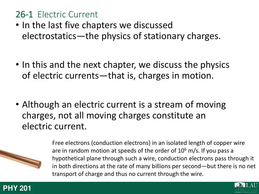
CHAPTER 26 Current and Resistance Electric Current 26-1 26-1 Electric Current PHY 201 • In the last five chapters we discussed electrostatics—the physics of stationary charges. • In this and the next chapter, we discuss the physics of electric currents—that is, charges in motion. • Although an electric current is a stream of moving charges, not all moving charges constitute an electric current. Free electrons (conduction electrons) in an isolated length of copper wire are in random motion at speeds of the order of 106 m/s. If you pass a hypothetical plane through such a wire, conduction electrons pass through it in both directions at the rate of many billions per second—but there is no net transport of charge and thus no current through the wire. 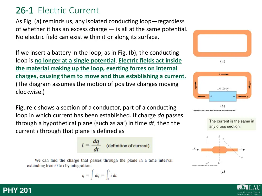26-1 Electric Current As Fig. (a) reminds us, any isolated conducting loop—regardless of whether it has an excess charge — is all at the same potential. No electric field can exist within it or along its surface. If we insert a battery in the loop, as in Fig. (b), the conducting loop is no longer at a single potential. Electric fields act inside the material making up the loop, exerting forces on internal charges, causing them to move and thus establishing a current. (The diagram assumes the motion of positive charges moving clockwise.) Figure c shows a section of a conductor, part of a conducting loop in which current has been established. 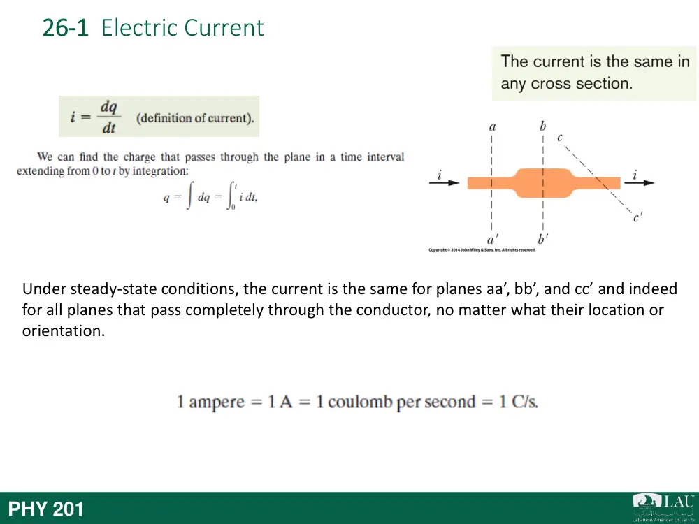If charge dq passes through a hypothetical plane (such as aa’) in time dt, then the current i through that plane is defined as (c) PHY 201 26-1 Electric Current PHY 201 Under steady-state conditions, the current is the same for planes aa’, bb’, and cc’ and indeed for all planes that pass completely through the conductor, no matter what their location or orientation. 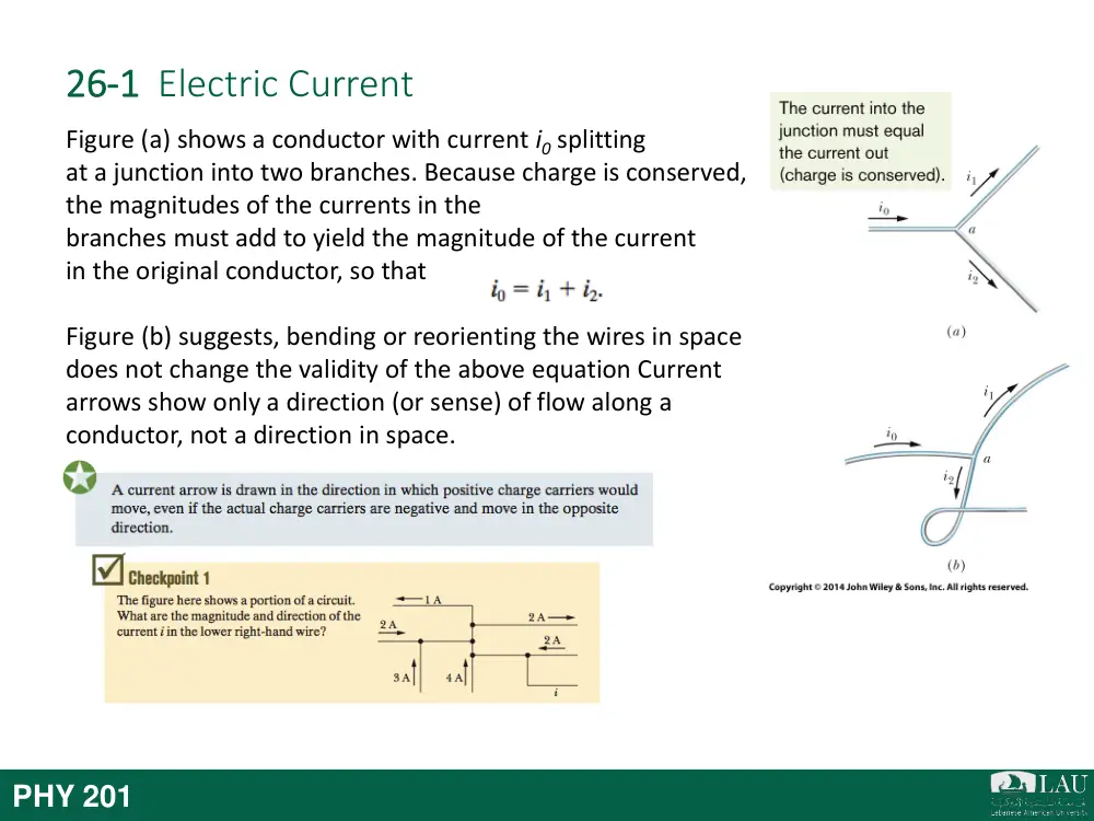26-1 Electric Current Figure (a) shows a conductor with current i0 splitting at a junction into two branches. Because charge is conserved, the magnitudes of the currents in the branches must add to yield the magnitude of the current in the original conductor, so that Figure (b) suggests, bending or reorienting the wires in space does not change the validity of the above equation Current arrows show only a direction (or sense) of flow along a conductor, not a direction in space. PHY 201 26-1 Electric Current Figure (a) shows a conductor with current i0 splitting at a junction into two branches. Because charge is conserved, the magnitudes of the currents in the branches must add to yield the magnitude of the current in the original conductor, so that Figure (b) suggests, bending or reorienting the wires in space does not change the validity of the above equation Current arrows show only a direction (or sense) of flow along a conductor, not a direction in space. 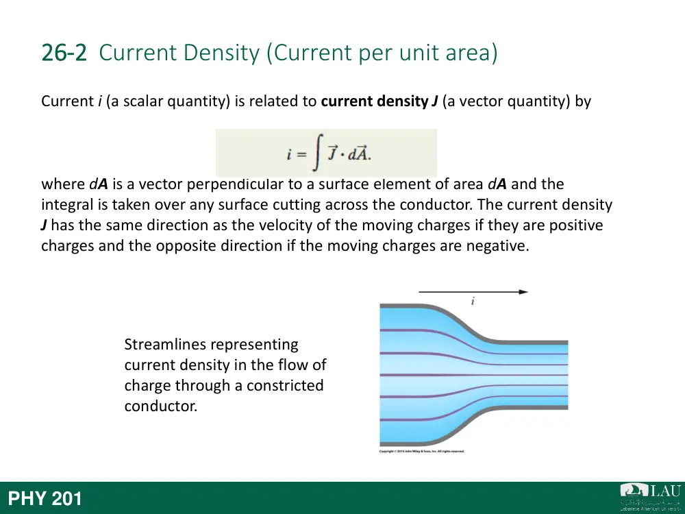Answer: 8A with arrow pointing right PHY 201 Electric Current 26-2 26-2 Current Density (Current per unit area) Current i (a scalar quantity) is related to current density J (a vector quantity) by where dA is a vector perpendicular to a surface element of area dA and the integral is taken over any surface cutting across the conductor. The current density J has the same direction as the velocity of the moving charges if they are positive charges and the opposite direction if the moving charges are negative. Streamlines representing current density in the flow of charge through a constricted conductor. 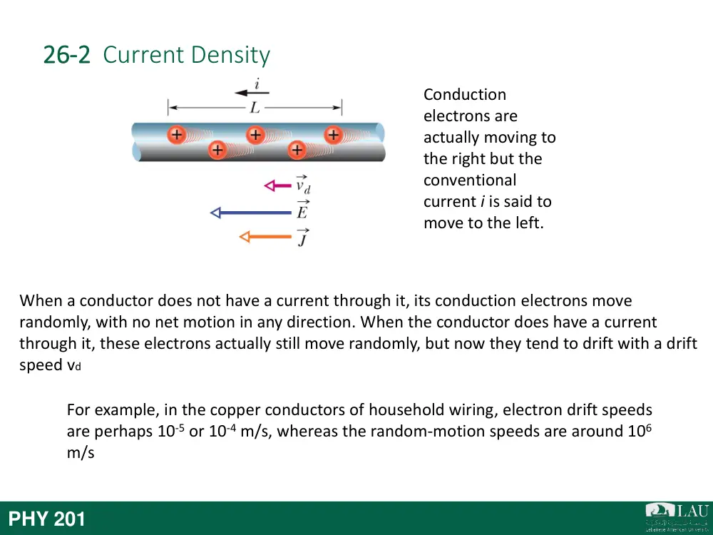PHY 201 26-2 Current Density Conduction electrons are actually moving to the right but the conventional current i is said to move to the left. PHY 201 When a conductor does not have a current through it, its conduction electrons move randomly, with no net motion in any direction. When the conductor does have a current through it, these electrons actually still move randomly, but now they tend to drift with a drift speed vd For example, in the copper conductors of household wiring, electron drift speeds are perhaps 10-5 or 10-4 m/s, whereas the random-motion speeds are around 106 m/s 26-2 Current Density Current is said to be due to positive charges that are propelled by the electric field. In the figure, positive charge carriers drift at speed vd in the direction of the applied electric field E which here is applied to the left. By convention, the direction of the current density J and the sense of the current arrow are drawn in that same direction, as is the drift speed vd. The drift velocity vd is related to the current density by Here the product ne, whose SI unit is the coulomb per cubic meter (C/m3), is the carrier charge density. Conduction electrons are actually moving to the right but the conventional current i is said to move to the left. PHY 201 Resistance and Resistivity 26-3 26-3 Resistance and Resistivity If we apply the same potential difference between the ends of geometrically similar rods of copper and of glass, very different currents result. The characteristic of the conductor that enters here is its electrical resistance. The resistance R of a conductor is defined as where V is the potential difference across the conductor and i is the current through the conductor. Instead of the resistance R of an object, we may deal with the resistivity ρ of the material: The reciprocal of resistivity is conductivity σ of the material: Assortment of Resistors PHY 201 A conductor whose function in a circuit is to provide a specified resistance is called a resistor Objects: Resistance Materials: Resistivity 26-3 Resistance and Resistivity PHY 201 26-3 Resistance and Resistivity PHY 201 This equation hold only for isotropic materials—materials whose electrical properties are the same in all directions 26-3 Resistance and Resistivity The resistance R of a conducting wire of length L and uniform cross section is Here A is the cross-sectional area. A potential difference V is applied between the ends of a wire of length L and cross section A, establishing a current i. The resistivity ρ for most materials changes with temperature. For many materials, including metals, the relation between ρ and temperature T is approximated by the equation Here T0 is a reference temperature, ρ0 is the resistivity at T0, and α is the temperature coefficient of resistivity for the material. The resistivity of copper as a function of temperature. PHY 201 Ohm’s Law 26-3 26-4 Ohm’s Law Figure (a) shows how to distinguish among devices. A potential difference V is applied across the device being tested, and the resulting current i through the device is measured as V is varied in both magnitude and polarity. Figure (b) is a plot of i versus V for one device. This plot is a straight line passing through the origin, so the ratio i/V (which is the slope of the straight line) is the same for all values of V. This means that the resistance R = V/i of the device is independent of the magnitude and polarity of the applied potential difference V. Figure (c) is a plot for another conducting device. Current can exist in this device only when the polarity of V is positive and the applied potential difference is more than about 1.5 V. When current does exist, the relation between i and V is not linear; it depends on the value of the applied potential difference V. PHY 201 26-4 Ohm’s Law I ~ V or I = V/R PHY 201 Bonus slide (not the exam)! - General relativity: The current description of gravitation in modern physics - Quantum Physics: The physics that governs the behavior of matter and light at the atomic (and subatomic) scale Good documentaries to watch: The Elegant Universe (Nova, PBS) PHY 201 Schrödinger's cat 26-4 Ohm’s Law A Microscopic View The assumption that the conduction electrons in a metal are free to move like the molecules in a gas leads to an expression for the resistivity of a metal: Here n is the number of free electrons per unit volume and τ is the mean time between the collisions of an electron with the atoms of the metal. Metals obey Ohm’s law because the mean free time τ is approximately independent of the magnitude E of any electric field applied to a metal. The gray lines show an electron moving from A to B, making six collisions en route. The green lines show what the electron’s path might be in the presence of an applied electric field E. Note the steady drift in the direction of -E. PHY 201 General Knowledge Power, Semiconductors, Superconductors 26-3 26-5 Power, Semiconductors, Superconductors Figure shows a circuit consisting of a battery B that is connected by wires, which we assume have negligible resistance, to an unspecified conducting device. The device might be a resistor, a storage battery (a rechargeable battery), a motor, or some other electrical device. The battery maintains a potential difference of magnitude V across its own terminals and thus (because of the wires) across the terminals of the unspecified device, with a greater potential at terminal a of the device than at terminal b. The power P, or rate of energy transfer, in an electrical device across which a potential difference V is maintained is If the device is a resistor, the power can also be written as or, PHY 201 26-5 Power, Semiconductors, Superconductors Semiconductors are materials that have few conduction electrons but can become conductors when they are doped with other atoms that contribute charge carriers. In a semiconductor, n (number of free electrons) is small (unlike conductor) but increases very rapidly with temperature as the increased thermal agitation makes more charge carriers available. This causes a decrease of resistivity with increasing temperature, as indicated by the negative temperature coefficient of resistivity for silicon in Table 26-2. Superconductors are materials that lose all electrical resistance below some critical temperature. Most such materials require very low temperatures, but some become superconducting at temperatures as high as room temperature. The resistance of mercury drops to zero at a temperature of about 4 K. PHY 201 26 Summary Current • The electric current i in a conductor is defined by Current Density • Current is related to current density by Eq. 26-1 Eq. 26-4 Resistance of a Conductor • Resistance R of a conductor is defined by • Similarly the resistivity and conductivity of a material is defined by • Resistance of a conducting wire of length L and uniform cross section is Eq. 26-8 Eq. 26-7 Eq. 26-10&12 Change of ρ with Temperature • The resistivity of most material changes with temperature and is given as Eq. 26-16 Eq. 26-17 Drift Speed of the Charge Carriers • Drift speed of the charge carriers in an applied electric field is related to current density by PHY 201 26 Summary Ohm’s Law • A given device (conductor, resistor, or any other electrical device) obeys Ohm’s law if its resistance R (defined by Eq. 26-8 as V/i) is independent of the applied potential difference V. Power • The power P, or rate of energy transfer, in an electrical device across which a potential difference V is maintained is • If the device is a resistor, we can write Eq. 26-26 Eq. 26-22 Eq. 26-27&28 Resistivity of a Metal • By assuming that the conduction electrons in a metal are free to move like the molecules of a gas, it is possible to derive an expression for the resistivity of a metal: PHY 201 CHAPTER 27 Circuits Electric Current 27-1 27-1 Single-Loop Circuits To produce a steady flow of charge, you need a “charge pump,” a device that—by doing work on the charge carriers—maintains a potential difference between a pair of terminals. We call such a device an emf device, and the device is said to provide an emf , which means that it does work on charge carriers. PHY 201 emf: electromotive force An emf device supplies the energy for the motion (of charge) via the work it does and thus maintain a potential difference between its terminal Emf devices: - Battery - Electric generator - Solar cells - Fuel cells - Human beings - Electric eels (600 V) Electric eels Hydrogen Fuel cells (Honda CFX clarity) Battery (Chevy Volt) Solar cells Figure shows an emf device (consider it to be a battery) that is part of a simple circuit containing a single resistance R. The emf device keeps one of its terminals (called the positive terminal and often labeled +) at a higher electric potential than the other terminal (called the negative terminal and labeled -). We can represent the emf of the device with an arrow that points from the negative terminal toward the positive terminal as in Figure. A small circle on the tail of the emf arrow distinguishes it from the arrows that indicate current direction. 27-1 Single-Loop Circuits PHY 201 27-1 Single-Loop Circuits An emf device does work on charges to maintain a potential difference between its output terminals. If dW is the work the device does to force positive charge dq from the negative to the positive terminal, then the emf (work per unit charge) of the device is An ideal emf device is one that lacks any internal resistance. The potential difference between its terminals is equal to the emf. A real emf device has internal resistance. The potential difference between its terminals is equal to the emf only if there is no current through the device. PHY 201 emf is the work per unit charge that the device does in moving charge from its low-potential terminal to its high-potential terminal. 27-1 Single-Loop Circuits Calculating Current in a Single-Loop Circuits After making a complete loop, our initial potential, as modified for potential changes along the way, must be equal to our final potential; that is, The value of Va cancels from this equation, which becomes Which gives us In the figure, let us start at point a, whose potential is Va, and mentally walk clockwise around the circuit until we are back at point a, keeping track of potential changes as we move. Our starting point is at the low-potential terminal of the battery. Because the battery is ideal, the potential difference between its terminals is equal to . When we pass through the battery to the high-potential terminal, the change in potential is + . Potential Method PHY 201 27-1 Single-Loop Circuits Calculating Current in a Single-Loop Circuits PHY 201 Also known as Kirchhoff’ loop rule 27-1 Single-Loop Circuits Internal Resistance Figure (a) shows a real battery, with internal resistance r, wired to an external resistor of resistance R. The internal resistance of the battery is the electrical resistance of the conducting materials of the battery and thus is an unremovable feature of the battery. Figure (b) shows graphically the changes in electric potential around the circuit. Now if we apply the loop rule clockwise beginning at point a, the changes in potential give us Solving for the current we find, PHY 201 27-1 Single-Loop Circuits Resistance in Series Figure (a) shows three resistances connected in series to an ideal battery with emf . The resistances are connected one after another between a and b, and a potential difference is maintained across a and b by the battery. The potential differences that then exist across the resistances in the series produce identical currents i in them. To find total resistance Req in Fig. (b), we apply the loop rule to both circuits. For Fig. (a), starting at a and going clockwise around the circuit, we find or For Fig. (b), with the three resistances replaced with a single equivalent resistance Req, we find or Equating them, we get, PHY 201 27-1 Single-Loop Circuits Resistance in Series PHY 201 27-1 Single-Loop Circuits Potential Difference Potential Difference across a real battery: In the Figure, points a and b are located at the terminals of the battery. Thus, the potential difference Vb - Va is the terminal-to-terminal potential difference V across the batter and is given by: Grounding a Circuit: Grounding a circuit usually means connecting one point in the circuit to a conducting path to Earth’s surface (actually to the electrically conducting moist dirt and rock below ground) Power of emf Device: The rate Pemf at which the emf device transfers energy both to the charge carriers and to internal thermal energy is PHY 201 Multiloop Circuits 27-2 27-2 Multiloop Circuits Figure shows a circuit containing more than one loop. If we traverse the left-hand loop in a counterclockwise direction from point b, the loop rule gives us If we traverse the right-hand loop in a counterclockwise direction from point b, the loop rule gives us If we had applied the loop rule to the big loop, we would have obtained (moving counterclockwise from b) the equation which is the sum of two small loops equations. PHY 201 27-2 Multi-Loop Circuits Figure (a) shows three resistances connected in parallel to an ideal battery of emf . . The applied potential difference V is maintained by the battery. Fig. b, the three parallel resistances have been replaced with an equivalent resistance Req. To derive an expression for Req in Fig. (b), we first write the current in each actual resistance in Fig. (a) as where V is the potential difference between a and b. If we apply the junction rule at point a in Fig. (a) and then substitute these values, we find If we replaced the parallel combination with the equivalent resistance Req (Fig. b), we would have and thus substituting the value of i from above equation we get, Resistances in Parallel PHY 201 27-2 Multi-Loop Circuits Resistance and capacitors PHY 201 27-3 The Ammeter and The Voltmeter An instrument used to measure currents is called an ammeter. To measure the current in a wire, you usually have to break or cut the wire and insert the ammeter so that the current to be measured passes through the meter. In the figure, ammeter A is set up to measure current i. It is essential that the resistance RA of the ammeter be very much smaller than other resistances in the circuit. Otherwise, the very presence of the meter will change the current to be measured. A meter used to measure potential differences is called a voltmeter. To find the potential difference between any two points in the circuit, the voltmeter terminals are connected between those points without breaking or cutting the wire. In the Figure, voltmeter V is set up to measure the voltage across R1. It is essential that the resistance RV of a voltmeter be very much larger than the resistance of any circuit element across which the voltmeter is connected. This is to insure that only a negligible current passes through the voltmeter, otherwise, the meter alters the potential difference that is to be measured. PHY 201 RC Circuits 27-3 27-4 RC Circuits Charging a capacitor: The capacitor of capacitance C in the figure is initially uncharged. To charge it, we close switch S on point a. This completes an RC series circuit consisting of the capacitor, an ideal battery of emf , and a resistance R. The charge on the capacitor increases according to in which C = q0 is the equilibrium (final) charge and RC=τ is the capacitive time constant of the circuit. During the charging, the current is And the voltage is: The product RC is called the capacitive time constant of the circuit and is represented with the symbol τ. Figure: RC circuit The plot shows the buildup of charge on the capacitor of the above figure. PHY 201 27-4 RC Circuits Discharging a capacitor: Assume now that the capacitor of the figure is fully charged to a potential V0 equal to the emf of the battery. At a new time t=0, switch S is thrown from a to b so that the capacitor can discharge through resistance R. When a capacitor discharges through a resistance R, the charge on the capacitor decays according to where q0 (=CV0) is the initial charge on the capacitor. During the discharging, the current is A plot shows the decline of the charging current in the circuit of the above figure. Figure: RC circuit PHY 201 27-3 RC Circuits PHY 201 A first order non-homogeneous differential equation: 𝑎 𝑑𝑞(𝑡) 𝑑𝑡 + 𝑏𝑞 𝑡 + 𝑐 = 0 where a,b,c are constants General solution: 𝑞 𝑡 = 𝐾𝑒−𝑏 𝑎𝑡 + 𝑐 𝑏 [𝑒−𝑏 𝑎𝑡 − 1] Charging a capacitor Capacitor Discharge Example: 𝑅 𝑑𝑞(𝑡) 𝑑𝑡 + 𝑞 𝑡 𝐶 − ℰ = 0 𝑖 = + 𝑑𝑞 𝑑𝑡 Example: 𝑅 𝑑𝑞(𝑡) 𝑑𝑡 + 𝑞 𝑡 𝐶 = 0 𝑖 = − 𝑑𝑞 𝑑𝑡 𝑅 = 𝑎 ; 𝑏 = 1 𝐶 ; 𝑐 = −ℰ 𝑅 = 𝑎 ; 𝑏 = 1 𝐶 ; 𝑐 = 0 Solution: 𝑞 𝑡 = 𝐾𝑒− 1 𝑅𝐶𝑡 − 𝐶ℰ[𝑒− 1 𝑅𝐶𝑡 − 1] Solution: 𝑞 𝑡 = 𝐾𝑒− 1 𝑅𝐶𝑡 𝑎𝑡 𝑡 = 0 𝑞 = 0 → 𝐾 = 0 𝑎𝑡 𝑡 = 0 𝑞 = 𝐶ℰ → 𝐾 = 𝐶ℰ 𝑞 𝑡 = 𝐶ℰ[1 − 𝑒− 1 𝑅𝐶𝑡] 𝑞 𝑡 = 𝐶ℰ 𝑒− 1 𝑅𝐶𝑡 Summary 27-4 27 Summary Emf • The emf (work per unit charge) of the device is Single-Loop Circuits • Current in a single-loop circuit: Eq. 27-1 Eq. 27-4 Series Resistance • When resistances are in series Eq. 27-7 Eq. 27-14 Eq. 27-24 RC Circuits • The charge on the capacitor increases according to • During the charging, the current is • During the discharging, the current is Eq. 27-33 Eq. 27-34 Power • The rate P of energy transfer to the charge carriers is • The rate Pr at which energy is dissipated as thermal energy in the battery is • The rate Pemf at which the chemical energy in the battery changes is Eq. 27-16 Eq. 27-17 Parallel Resistance • When resistances are in parallel Eq. 27-40 PHY 201 Wheatstone Bridge 27+ History • The Wheatstone Bridge was invented in 1833 by Samuel Hunter Christie • Later named after Sir Charles Wheatstone for his many applications of the circuit through the 1840s • The most common procedure for the bridge remains the testing of unknown electrical resistance PHY 201 How Does it Work? • Uses ratio of 3 known resistors • Measures fourth unknown resistance • Balanced voltage between point 1 and battery’s negative, and between point 2 and battery’s negative allows the measurement : http://www.opamp- electronics.com/tutorials/bridge_circuits_1_08_10.htm PHY 201 How Does it Work? : http://www.opamp- electronics.com/tutorials/bridge_circuits_1_08_10.htm PHY 201 If the ratio of the two resistances (R2 / R1) is equal to the ratio of the two (Rx / R3), then the voltage between the two midpoints (B and D) will be zero and no current will flow through the galvanometer How Does it Work? : http://www.opamp- electronics.com/tutorials/bridge_circuits_1_08_10.htm PHY 201 Kirchhoff's rule is used for finding the voltage in the loops ABD and BCD When the bridge is balanced, then IG = 0, so the second set of equations can be rewritten as: I3 = Ix and I1 = I2 How is it used? • Main focus of the Wheatstone Bridge = applications using electricity • The circuit monitors sensor devices like strain gauges – it reads the level of the strain in the system • The galvanometer measures whether the gauges are balanced or not • Electrical power distributors use the Wheatstone Bridge to locate breaks in the power lines PHY 201