EECE 340 Chapter 10, Fall 2011

Chapter 10 Discrete-Time Signals and Systems Introduction � A discrete-time signal x(nTs) is a signal that is only defined at discrete instants of time. A discrete-time signal is usually derived from a continuous time signal through sampling and Ts is called the sampling period. Therefore, sampling the signal x(t) at time Ts yields a discrete-time signal x(nTs). 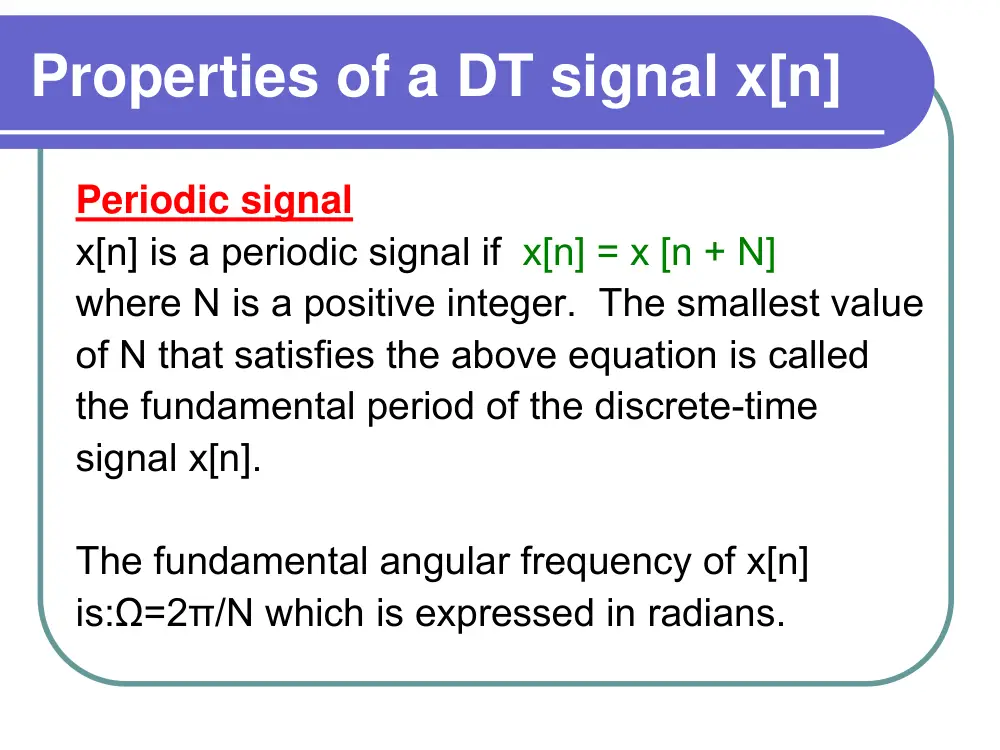For convenience of presentation, we use x[n] = x(nTs) for n = 0, ± 1, ±2, ±3, …… Properties of a DT signal x[n] Periodic signal x[n] is a periodic signal if x[n] = x [n + N] where N is a positive integer. The smallest value of N that satisfies the above equation is called the fundamental period of the discrete-time signal x[n]. The fundamental angular frequency of x[n] is:Ω=2π/N which is expressed in radians. 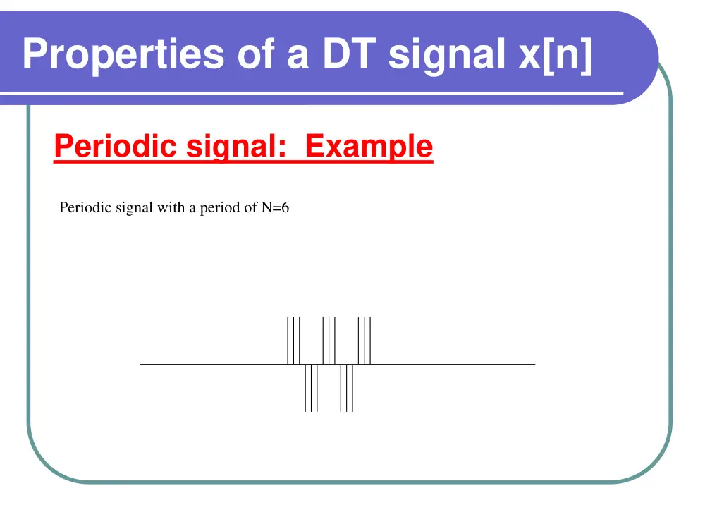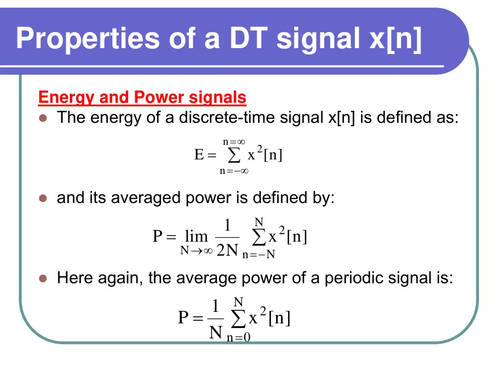Properties of a DT signal x[n] Periodic signal: Example Periodic signal with a period of N=6 Properties of a DT signal x[n] Periodic signal: Examples For each of the following signals determine whether it is periodic or not � x[n]=cos(2n), Not Periodic � x[n]=cos(2πn), Periodic with N=1 � x[n]=(-1)n, Periodic with N=2 � x[n]=(-1)n2, Periodic with N=2 Properties of a DT signal x[n] Energy and Power signals � The energy of a discrete-time signal x[n] is defined as: � and its averaged power is defined by: � Here again, the average power of a periodic signal is: ∑ ∞ = =−∞ = n n 2 x [n] E ∑ =− →∞ = N N n 2 N x [n] 2N 1 lim P ∑ = = N 0 n 2 x [n] N 1 P Properties of a DT signal x[n] 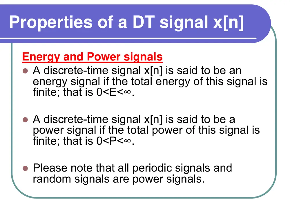Energy and Power signals � A discrete-time signal x[n] is said to be an energy signal if the total energy of this signal is finite; that is 0<E<∞. � A discrete-time signal x[n] is said to be a power signal if the total power of this signal is finite; that is 0<P<∞. � Please note that all periodic signals and random signals are power signals. 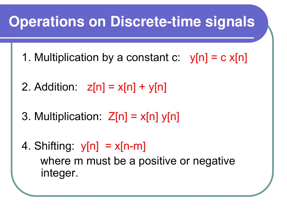Operations on Discrete-time signals 1. Multiplication by a constant c: y[n] = c x[n] 2. Addition: z[n] = x[n] + y[n] 3. Multiplication: Z[n] = x[n] y[n] 4. Shifting: y[n] = x[n-m] where m must be a positive or negative integer. 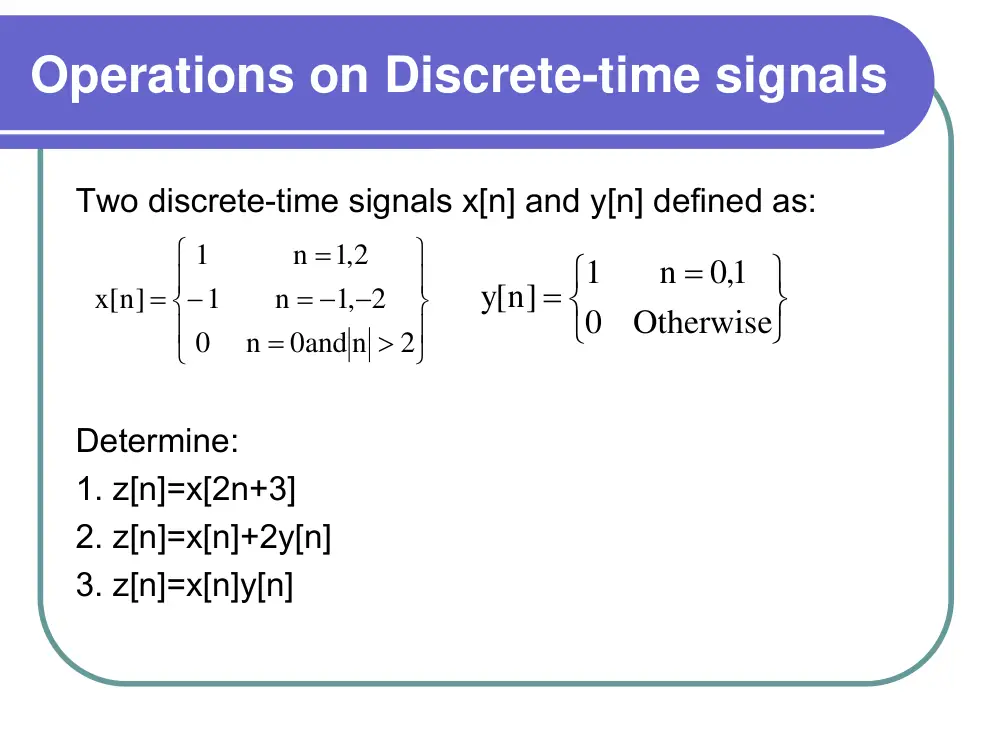Operations on Discrete-time signals Two discrete-time signals x[n] and y[n] defined as: Determine: 1. z[n]=x[2n+3] 2. z[n]=x[n]+2y[n] 3. 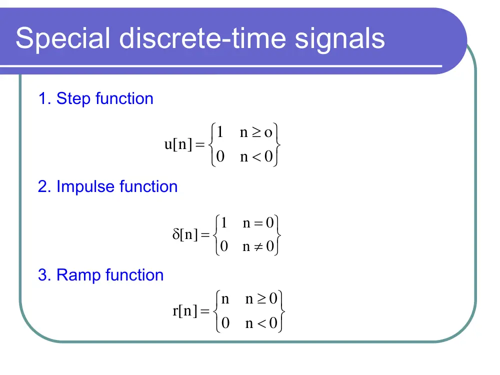z[n]=x[n]y[n] ⎪⎭ ⎪⎬ ⎫ ⎪⎩ ⎪⎨ ⎧ > = = − − − = = 2 0and n n 0 ,1 2 n 1 2,1 n 1 x[n] ⎭ ⎬ ⎫ ⎩ ⎨ ⎧ = = Otherwise 0 1,0 n 1 [y n] Special discrete-time signals 1. Step function 2. Impulse function 3. Ramp function ⎭ ⎬ ⎫ ⎩ ⎨ ⎧ < ≥ = 0 n 0 o n 1 [n] u ⎭ ⎬ ⎫ ⎩ ⎨ ⎧ ≠ = = δ 0 n 0 0 n 1 n] [ ⎭ ⎬ ⎫ ⎩ ⎨ ⎧ < ≥ = 0 n 0 0 n n [r n] Discrete time systems � A discrete-time system is viewed as an interconnection of operations that transforms an input signal into an output signal. � In general, the input-output relation of a discrete time system is described by: ∑ ∞ = − ρ = 0 k k k] x[n [y n] Discrete time systems: Example ( 2 )] x[n ]1 x[n 3 x[n] 1 [y n] − + − + = Delay; S Delay; S + x[n] y[n] 1/3 1/3 1/3 Properties of a discrete-time system Stable system A discrete-time system represented by: is said to be stable iff ∑ ∞ = − ρ = 0 k k k] x[n n] [y ρ <1 Properties of a discrete-time system Causality A discrete-time system is causal if the present value of the output signal depends only on the present or past values of the input signal Examples � y[n] = x[n] + x[n-1] + x[n-4] is a causal system � y[n] = x[n+1] + x[n]+x[n-3] is not a causal system. Properties of a discrete-time system Linearity A discrete-time system is linear if the two properties apply: Superposition and homogeneity. Example: y[n] = n x[n] Properties of a discrete-time system Time-invariant A shift in the input corresponds to the same shift in the output. Example Y[n]=nx[n] Impulse response of a discrete-time system � The impulse response h[n] of a discrete- time system is easily obtained by setting the input signal to the impulse δ[n] . Input-output relation of an LTI system: The convolution sum Consider a LTI discrete-time system with input x[n] and impulse response h[n]. The output of the signal is written as the convolution sum The sum above is termed the convolution sum and is denoted by the symbol *; that is, y[n] = x[n]*h[n] h[n] x[n] y[n] ∑ ∞ = −∞ = − = k k k] x[k]h[n [y n] Example Consider the discrete-time LTI system model representing a two-path propagation channel. If the strength of the indirect path is a = 1/2, then determine the output of this system if the input is: ]1 2 x[n 1 x[n] [y n] − + = ⎪ ⎪ ⎭ ⎪⎪ ⎬ ⎫ ⎪ ⎪ ⎩ ⎪⎪ ⎨ ⎧ = − = = = Otherwise 0 2 n 2 1 n 4 0 n 2 x[n] Convolution Sum Evaluation Procedure 1.The first step is to determine the impulse response h[n] 2. Write x[n] as the weight sum of time shifted impulses 3. Compute h[n]*x[n]. ]1 2 [n 1 [n] h[n] − δ + δ = 2] 2 [n ]1 4 [n 2 [n] x[n] − − δ − + δ = δ First Method In this method, the basic definition of the convolution of two finite causal sequences (The sequence has zero value for negative values of n) is used with the fact that the convolution of an M-point sequence x[n] and an N- point sequence h[n] is an (M+N-1)-point sequence y[n]. In a mathematical form, k ] h[k]x[n [y n] M 1 N 0 k∑ − + = − = Second Method In this method, the convolution sum y[n] of the two finite sequences h[n] and x[n] is given by: y[n]= h[0]x[n]+h[1]x[n-1]+... +h[k]x[n-k]+...+h[m]x[n-m] m is the highest index for which h[m] is different than zero. Third Method This method uses the approach discussed in: � J.W. Pierre, “A Novel Method for Calculating the Convolution Sum of Two Finite Length Sequences”, IEEE Transactions on Education, Vol. 39, No.1, pp.77- 80, February 1996. Third Method This procedure is similar to the multiplication of two decimal numbers which makes this method attractive, easy to learn, and simple to implement. To obtain this table, the following steps are done: n 0 1 2 3 4 5 k h[k] x[n] 2 4 -2 0 1 x[n-1] 2 4 -2 1 0.5 h[0]x[n] 2 4 -2 h[1]x[n-1] 0 1 2 -1 y[n] 2 5 0 -1 Example The output y[n] of the four-point moving-average system is related to the input x[n] according to the formula → Determine the output y[n] when the input is the rectangular pulse defined as x[n] = u[n] - u[n - 10] ]3 4 [n 1 2] 4 [n 1 ]1 4 [n 1 4 [n] 1 h[n] − δ + − δ + − δ + δ = ∑ = − = 3 k 0 k] x[n 4 1 n] [y [n -9] [n -8] [n -7] 6 ] [n 5] [n 4] [n ]3 [n 2] [n ]1 [n [n] x[n] + δ + δ + δ − δ + − + δ − + δ − + δ − + δ − + δ = δ � n 0 1 2 3 4 5 6 7 8 9 10 11 12 k h[k] x[n] 1 1 1 1 1 1 1 1 1 1 0 ¼ x[n-1] 1 1 1 1 1 1 1 1 1 1 1 ¼ x[n-2] 1 1 1 1 1 1 1 1 1 1 2 ¼ x[n-3] 1 1 1 1 1 1 1 1 1 1 3 ¼ h[0]x[n] ¼ ¼ ¼ ¼ ¼ ¼ ¼ ¼ ¼ ¼ h[1]x[n-1] ¼ ¼ ¼ ¼ ¼ ¼ ¼ ¼ ¼ ¼ h[2]x[n-2] ¼ ¼ ¼ ¼ ¼ ¼ ¼ ¼ ¼ ¼ h[3]x[n-3] ¼ ¼ ¼ ¼ ¼ ¼ ¼ ¼ ¼ ¼ y[n] ¼ ½ ¾ 1 1 1 1 1 1 1 3/4 ½ ¼ Example � In summary, ⎪ ⎪ ⎭ ⎪⎪ ⎬ ⎫ ⎪ ⎪ ⎩ ⎪⎪ ⎨ ⎧ ≤ ≤ − ≤ ≤ ≤ ≤ + = 12 n 10 4 n 13 9 n 4 1 3 n 0 4 1 n [y n] Relations between LTI System Properties and the Impulse Response � The impulse response completely characterizes the input-output behavior of an LTI system. Hence, properties of the system, such as memory, causality, and stability, are related to the system's impulse response. In this section, we explore the relationships involved. Memoryless LTI systems � The output of a memoryless LTI system depends only on the current input. How this property is related to h[n]? � For an LTI system, y[n] = h[n] * x[n] = � For this system to be memoryless, y[n] must depend only on x[n] and therefore cannot depend on x[n - k] for k#0. Hence, all other terms must be zero except h[0]x[n]. � This condition implies that h[k] = 0 for k#0; thus, a discrete-time LTI system is memoryless if and only if where c is an arbitrary constant. Other terms x[n]h[0] k] [k]h[n x k k + = − ∑ ∞ = −∞ = c [n] h[n] = δ Causal LTI Systems � The output of a causal LTI system depends only on past or present values of the input. Again, we write the convolution sum as: y[n] = ... + h[-2]x[n + 2] + h[-l]x[n + 1] + h[O]x[n] + h[l]x[n - 1] + h[2]x[n - 2] +…. � We see that past and present values of the input, x[ n], x[n - 1], x[n - 2],..., are associated with indices k≥ 0 in the impulse response h[ k], while future values of the Input, x[ n + 1], x[ n + 2], . . ., are associated with indices k < 0. � In order, then, for y[ n] to depend only on past or present values of the input, we require that h[k] = 0 for k < 0. Stable LTI Systems � An LTI DT system is stable iff the output is bounded for every bounded input. � A bounded output means: When � If we assume that the output is bounded for every bounded input, then M k] h[k]x[n h[n] x[n] n] [y k k < − = ∗ = ∑ ∞ = −∞ = < ∞ ≤ Mx [n] x < ∞ ≤ ∑ ∞ = =−∞ x y k k M M h[k] Example A first-order DT system is described by the difference equation y[n]=ρy[n-1]+x[n]. and has the impulse response h[n]=ρnu[n]. 1. Is this system causal? Yes 2. Is the system memoryless? No 3. Is it BIBO stable? Yes if |ρ|<1. Problem For each of the following impulse responses, determine whether the corresponding system is (i) memoryless, (ii) causal, and (iii) stable. Justify your answers. � (a) h[n] = 2nu[-n] not memoryless, not causal, stable � (b) h[n] =e2n u[n - 1] not memoryless, causal, not stable � (c) h[n] = (0.5)n u[n] not memoryless, causal, stable Step-response � Step input signals are often used to characterize the response of an LTI system to sudden changes in the input. The step response is defined as the output due to a unit step input signal. Let h[ n] be the impulse response of a discrete-time LTI system, and denote the step response as s[ n]. We thus write � That is, the step response is the running sum of the impulse response. Note that we may invert these relationships to express the impulse response in terms of the step response as h[n] = s[n] - s[n - 1] ∑ ∑ −∞ = ∞ = =−∞ = − = ∗ = n k k k h[k] k] h[k]u[n h[n] u[n] [s n] EXAMPLE Find the step response of the first-order recursive system with impulse response assuming that |ρ| < 1. Answer: u[n] h[n] ρn = u[n] 1 1 n] [s 1 n − ρ − ρ = + Difference Equation Representations of LTI Systems � Linear constant-coefficient difference equations provide another representation for the input-output characteristics of LTI systems. Difference equations are used to represent discrete-time systems, while differential equations represent continuous-time systems. A linear constant-coefficient difference equation has a similar form of that of continuous system, with the derivatives replaced by delayed values of the input x[ n ] and output y[n]: � Examples: An example of a second-order difference equation is y[n] + y[n - 1] + 4y[n - 2] = x[n] + 2x[n - 1] Solving Difference Equations � This is best done with the use of the z- transform discussed later. Block Diagram Representations � In this section, we examine block diagram representations of LTI systems described by difference equations. A block diagram is an interconnection of elementary operations that act on the input signal. The block diagram is a more detailed representation of a system than the impulse response or difference equation, on descriptions, since it describes how the system's internal computations or operations are ordered. � Block diagram representations consist of an interconnection of three elementary operations on signals: 1. Scalar multiplication: y[n] = cx[n], where c is a scalar. 2. Addition: y[n] = x[n] + w[n]. 3. Time shift for that discrete-time LTI systems: y[n] = x[n - 1]. Direct Form I: Example 1. Let us rewrite the above equation in a manner similar to that of the continuous system 2. The above equation can be written in the following form with 2] b x[n ]1 b x[n b x[n] 2] [y n a ]1 [y n a [y n] 2 1 0 2 1 − + − + = − + − + 2] b x[n ]1 b x[n b x[n] 2] [y n a ]1 [y n a [y n] 2 1 0 2 1 − + − + + − − − − = w[n] 2] [y n a ]1 [y n a [y n] 2 1 + − − − − = 2] b x[n ]1 b x[n b x[n] w[n] 2 1 0 − + − + = Direct Form I: Example 3. Draw the block diagram of the two quantities then connect as shown below Direct Form II: Example We may view Direct Form I as a cascade the of two systems: one with input x[n] and output w[n] and a second with input w[ n] and output y[n]. Since these are LTI systems, we may interchange their order without changing the input-output behavior of the cascade. State Variable representation of Discrete LTI Systems � We shall develop the general state- variable description by starting with the direct form II implementation of a second-order LTI system. Procedure is almost the same as for the case of a continuous system. The output of each time delay is denoted by a state q[n] as shown in the next example Example Example: Matrix Format