EECE 340 Chapter 15, Fall 2011

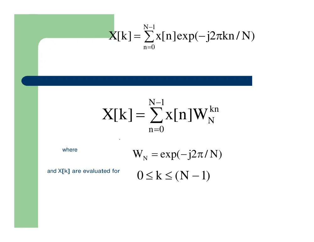
Chapter 15 FFT Algorithms FFT Algorithms � Highly efficient algorithms for computing the DFT were first developed in the 1960s. � All Fast Fourier Transforms (FFTs) rely upon the fact that the standard DFT involves redundant calculation. ∑ − = π − = 1 N n 0 kn / N) 2j x[n]exp( [k] X ∑ − = = 1 N 0 n kn x[n]WN [k] X where / N) 2j exp( WN π − = and X[k] are evaluated for )1 (N k 0 − ≤ ≤ . Periodic Nature of the function � Before getting down to detail, you may find it helpful if we demonstrate the periodic nature of . For simplicity let us consider a short DFT - say N=8. 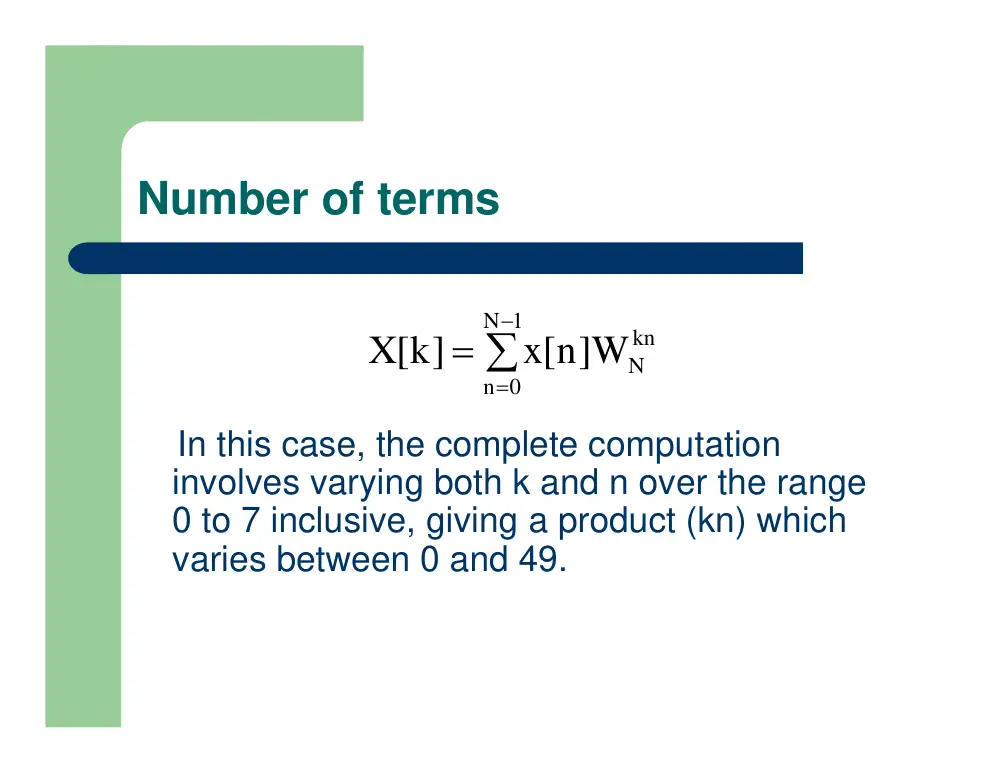nk N W nk WN Number of terms In this case, the complete computation involves varying both k and n over the range 0 to 7 inclusive, giving a product (kn) which varies between 0 and 49. 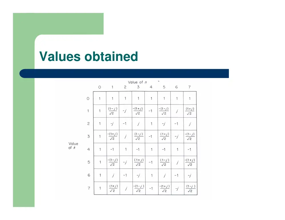∑ − = = 1 N 0 n kn x[n]WN X[k] Values obtained Observations � There are only eight distinct values. � Half the values are the negative of the other half, we might say that there are only four distinct values. � The table forms a matrix with diagonal symmetry. Furthermore, many of the values are +1 or -1, implying simple additions and subtractions. 2 Algorithms will be presented - The Conventional Decomposition Method - The index-Mapping Method It is important to understand that conventional decomposition and index-mapping are two ways of looking at the same problem. There is no essential difference between them. In Both Methods, we require N=2i, where i is an integer Conventional decomposition � Conventional decomposition may be introduced by considering a signal x[n] broken down into shorter, interleaved, subsequences. The process is referred to as decimation-in- time, and gives rise to one of the major classes of FFT algorithm. � Suppose we have a signal with N sample values, where N is an integer power of 2. We first separate x[n] into two subsequences, each with N/2 samples. The first subsequence consists of the even-numbered points in x[n], and the second consists of the odd-numbered points. Writing n=2r when n is even, and n=2r+l when n is odd, the DFT may be recast as: Procedure ( ) ( ) ∑ ∑ ∑ ∑ ∑ − = = − = + = − = + + = + + = ≤ ≤ = N / 2) 1 ( 0 r 2 rk N k N -1 (N/2) 0 r 2 rk N N / 2) 1 ( 0 r )1 k (2r N -1 (N/2) 0 r 2rk N 1 N 0 n nk N ]1 W x[2r W x[2r] W ]1 W x[2r x[2r]W N -1 k 0 x[n]W X[k] N / 2 2 N W / N) exp( 2 2j W = π − = ( ) ( ) G[k] W H[k] ]1 W x[2r W x[2r] W [k] X k N N / 2) 1 ( 0 r rk N / 2 k N -1 (N/2) 0 r rk N/2 + = + + = ∑ ∑ − = = ( ) ( ) ∑ ∑ − = = + + = N / 2 ) 1 ( 0 r rk 2 N k N -1 (N/2) 0 r rk 2 N 1] W x[2 r W W x[2r] X [k ] Conclusion � If we assume that the transform length N is an integer power of 2, it follows that N/2 is even. Therefore we can take the decomposition further, by breaking each N/2-point subsequence down into two shorter, N/4-point sub-sequences. The process can continue until, in the limit, we are left with a series of 2-point subsequences, each of which requires a very simple 2-point DFT. A complete decomposition of this type gives rise to one of the commonly-used radix-2, decimation-in-time, FFT algorithms. Example � We can demonstrate the decimation-in-time process quite easily in the case of a short transform - for example, N=8. The signal x[n] is defined for: n = {0 1 2 3 4 5 6 7} � We start by forming two subsequences of the even- numbered and odd-numbered points: n = {0 2 4 6} and {1 3 5 7} � Each subsequence is further decimated, giving: n = {0 4} and (2 6} and {1 5}, and {3 7} Conclusion � The 8-point DFT is now realized as four 2- point DFTs, performed on pairs of sample values separated by half the transform length. Thus x[0] is paired with x[4], x[2] is paired with x[6], and so on. Although the original DFT has been recast in terms of a series of 2-point DFTs, we must be careful not to assume that the resulting computation is trivial. Index-Mapping Method Procedures � The index-mapping approach may be introduced as follows. We start by expressing the transform length N as the product of two factors N1 and N2: . N = N1 N2 � We also define two new indices: 1 ,0 1, 2, ..., N n 1 1 − = 1 ,0 1, 2, ..., N n 2 2 − = Computation of n � The following linear equation may now be used to map the values of and into the time- index n of the DFT: � where M1 and M2 are constants, and the brackets and subscript N denote modulo-N. 2 N 2 1 1 M n ) (M n n + = Example � Let us begin with a simple example - a 4-point DFT which we will decompose into 2-point DFTs. We can use it to illustrate many important features of FFT algorithms, and to introduce further terminology. In this case N=4 and N1=N2=2. For reasons which will become clear as we proceed, we choose M1=2, M2=1. � Hence: n = 2n1 + n2 The mappings of n n = 2n1 + n2 The DFT for N=4 is given by: X[k]= ∑ ∑ = − = = 3 0 n nk 4 1 N 0 n kn N x[n]W [n]W x ∑ ∑ = + = = 1 0 n n ) k(2n 4 2 1 1 0 n 2 2 1 1 x[n ,n ]W [k] X ∑ ∑ = = = 1 0 n kn 4 2kn 4 2 1 1 0 n 2 2 1 1 W x[n ,n ]W [k] X ∑ ∑ ∑ ∑ = = = = + = = 1 0 n 2kn 4 1 k 4 1 0 n 2kn 4 1 1 0 n 2kn 4 2 1 1 0 n kn 4 1 1 1 1 1 1 2 2 ]1, W x[n W x[n 0, ]W x[n ,n ]W W X[k] � Let us examine the last equation a little more carefully. Referring to the index map for n, we see that if n2=0, then n=0, 2 when nl=0, 1; and if n2=1 then n=l, 3 when nl=0, 1. Hence: � Therefore one of the 2-point DFTs involves pairing x[0] and x[2]; the other involves pairing x[1] and x[3]. Once again, we see that the decimation creates pairs of sample values separated by half the transform length. ∑ ∑ = = + = 1 0 n 2kn 4 1 k 4 1 0 n 2kn 4 1 1 1 1 1 ]1, W x[n W x[n 0, ]W [k] X [ 2k ] 4 k 4 2k 4 x[3]W x ]1[ W x[2]W x[0] X[k] + + + = [ 2 ] 4 1 4 2 4 x[3]W W x ]1[ x[2]W } {x[0] X ]1[ + + + = [ 0 ] 4 2 4 0 4 x[3]W x ]1[ W x[2]W } {x[0] X[2] + + + = [ 2 ] 4 3 4 2 4 x[3]W W x ]1[ x[2]W } {x[0] X[3] + + + = [ 0 ] 4 0 4 0 4 x[3]W W x ]1[ x[2]W } {x[0] X[0] + + + = [ 2k ] 4 k 4 2k 4 x[3]W x ]1[ W x[2]W x[0] X[k] + + + = This way of representing a 4-point DFT may be visualized the help of the signal flow graph in the Figure below. Example An 8-pomt, radix-2, decimation in time, in-place, FFT may be defined by the following index-map equations all six independent variables taken over the range 0 to 1. � Construct index maps for n. Assuming, a natural-order output, specify the shuffled input sequence. � Draw a signal flow graph for the FFT, expressing all branch transmittances as powers of � Redraw the flow graph in terms of basic (2-point) FFT butterflies and twiddle factors. How many complex multiplications, are required by the FFT? 3 2 1 n 2n 4n n + + = W8 Solution 1 n 2 n 3 n n 0 0 0 0 1 0 0 4 0 1 0 2 1 1 0 6 0 0 1 1 1 0 1 5 0 1 1 3 1 1 1 7 b. The form of the DFT for N=8 X[k]= ∑ ∑ = − = = 7 0 n nk 8 1 N 0 n kn N x[n]W [n]W x ∑ ∑ ∑ = + + = = = 1 0 n n ) 2n k(4n 8 3 2 1 1 0 n 1 0 n 3 3 2 1 2 1 x[n ,n ,n ]W [k] X ∑ ∑ ∑ = = = = 1 0 n 4kn 8 3 2 1 1 0 n 2kn 8 1 0 n kn 8 1 1 2 2 3 3 x[n ,n ,n ]W W W X[k] ⎟⎟ ⎠ ⎞ ⎜⎜ ⎝ ⎛ + + ⎟⎟ + ⎠ ⎞ ⎜⎜ ⎝ ⎛ + + = + + = = ∑ ∑ ∑ ∑ ∑ ∑ ∑ ∑ ∑ ∑ = = = = = = = = = = 1 0 n 4kn 8 2 1 1 0 n 2kn 8 1 8 1 0 n 4kn 8 2 1 1 0 n 2kn 8 0 8 1 0 n 4kn 8 3 2 1 1 0 n 2kn 8 1 0 n kn 8 1 0 n 4kn 8 3 2 1 1 0 n 2kn 8 1 0 n kn 8 1 1 2 2 1 1 2 2 1 1 2 2 3 3 1 1 2 2 3 3 ]1 W 2n x[4n W W 0]W 2n x[4n W W [k] X n ]W 2n x[4n W W [k] X x[n ,n ,n ]W W W X[k] ⎟⎟ ⎠ ⎞ ⎜⎜ ⎝ ⎛ + + ⎟⎟ + ⎠ ⎞ ⎜⎜ ⎝ ⎛ + + ⎟⎟ ⎠ ⎞ ⎜⎜ ⎝ ⎛ + ⎟⎟ + ⎠ ⎞ ⎜⎜ ⎝ ⎛ = ⎟⎟ ⎠ ⎞ ⎜⎜ ⎝ ⎛ + + ⎟⎟ + ⎠ ⎞ ⎜⎜ ⎝ ⎛ + + = ∑ ∑ ∑ ∑ ∑ ∑ ∑ ∑ = = = = = = = = 1 0 n 4kn 8 1 2k 8 1 8 1 0 n 4kn 8 1 0 8 1 8 1 0 n 4kn 8 1 2k 8 0 8 1 0 n 4kn 8 1 0 8 0 8 1 0 n 4kn 8 2 1 1 0 n 2kn 8 1 8 1 0 n 4kn 8 2 1 1 0 n 2kn 8 0 8 1 1 1 1 1 1 1 1 1 1 2 2 1 1 2 2 ]1 W 2 x[4n W W ]1 W x[4n W W 2]W x[4n W W x[4n ]W W W [k] X ]1 W 2n x[4n W W 0]W 2n x[4n W W X[k] [ ] ( ) [ ] ( ) [ ] ( ) [ ] ( 4k ) 8 0 8 2k 8 1 8 4k 8 0 8 0 8 1 8 4k 8 0 8 2k 8 0 8 4k 8 0 8 0 8 0 8 1 0 n 4kn 8 1 2k 8 1 8 1 0 n 4kn 8 1 0 8 1 8 1 0 n 4kn 8 1 2k 8 0 8 1 0 n 4kn 8 1 0 8 0 8 x[7]W x[ ]3 W W W x[5]W W W x ]1[ W x[6]W x[2]W W W x[4]W W W x[o]W [k] X ]1 W 2 x[4n W W ]1 W x[4n W W 2]W x[4n W W x[4n ]W W W [k] X 1 1 1 1 1 1 1 1 + + + + + + + = ⎟⎟ ⎠ ⎞ ⎜⎜ ⎝ ⎛ + + ⎟⎟ + ⎠ ⎞ ⎜⎜ ⎝ ⎛ + + ⎟⎟ ⎠ ⎞ ⎜⎜ ⎝ ⎛ + ⎟⎟ + ⎠ ⎞ ⎜⎜ ⎝ ⎛ = ∑ ∑ ∑ ∑ = = = =